Tags: Magnetostatic Potential / Legendre Polynomials / Boundary Conditions
![]() Using the magnetostatic potential can be extremely useful to calculate magnetostatic problems. However, it can only be defined if no currents are present. In this problem you will discover how we can still use the potential in situations of strongly confined surface currents.
Using the magnetostatic potential can be extremely useful to calculate magnetostatic problems. However, it can only be defined if no currents are present. In this problem you will discover how we can still use the potential in situations of strongly confined surface currents.
Problem Statement
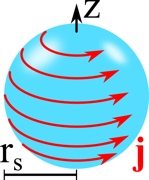 Consider a sphere with relative permeability μr and radius rs.
On the surface of the sphere there shall be a current flowing in azimuthal φ-direction, strongest at the equator:
\[\mathbf{j}\left(\mathbf{r}\right)=j_{0}\delta\left( r-r_{s} \right)\sin\theta\mathbf{e}_{\varphi}\]
Calculate the magnetic induction B(r) everywhere.
Discuss what further steps you would have to take if the surface current obeys a more complicated form.
Background: Artificial Magnetic Materials
In the optical frequency range, magnetic light-matter-interactions are usually very weak. This means that relative permeabilities μr are very close to unity.
Nevertheless, strong magnetic interactions would have a lot of incredible applications like perfect lenses or cloaking devices. The reason is that such devices rely on a spatially varying permittivity ε(r,ω) and permeability μ(r,ω).
Hence, there is a lot of interest to design artificial materials that have a somewhat stronger magnetic interaction than ordinary matter.
One way to get such an artificial magnetic material is described in the publication "Self-Assembled Plasmonic Core–Shell Clusters with an Isotropic Magnetic Dipole Response in the Visible Range" by Mühlig et al., ACS Nano 5 (2011).
In this paper, the authors attach a lot of small metallic nanospheres with radii around 10 nm onto a larger dielectric sphere with a radius of around 100 nm.
The metallic spheres then act as an effective medium that can have an extremely high permittivity at certain frequencies. Then, an excitation field causes the electrons in the metal to oscillate around the magnetic field vector. This (oscillating!) ring current leads to an effective coupling to the magnetic field. In a certain sense, we ask in our problem for the inverse situation: What kind of magnetic field is caused by a certain azimuthal surface current?
Hints
If there is no current j(r), we can usually employ the magnetostatic potential Ψ(r). Here, we have a current distribution that is nonvanishing only at the surface r = rs.
So we can express the fields in terms of Ψ(r) everywhere except on the surface of the sphere. So, can we use the boundary conditions to find relations between the fields in- and outside of the sphere?
Let's find the magnetic field for this special spherical current!
The solution of the problem can be found straight forward. First of all, we have to find what this special surface current implies for the fields in- and outside of the sphere. Then, we will use the magnetostatic potential to express the fields in both regions. Connecting both information we will be able to find the magnetic induction.
Solution: Magnetic field of a sphere with surface current
Boundary Conditions
Starting from Gauss's law for magnetism, \(\nabla\cdot\mathbf{B} \left(\mathbf{r}\right)=0\)
and Ampères law, \(\nabla\times\mathbf{H}\left(\mathbf{r}\right)=\mathbf{j}\left(\mathbf{r}\right)\),
we know that the normal part of the magnetic induction is continuous and the tangential part of the magnetic field makes a jump because of the present current.
Because of the spherical symmetry, we might express both conditions using the radial unit vector \(\mathbf{e}_{r}\):
\[\begin{eqnarray*}\mathbf{e}_{r}\cdot\left(\mathbf{B}_{\mathrm{out}}\left(r=r_{s,}\theta,\varphi\right)-\mathbf{B}_{\mathrm{in}} \left(r=r_{s,}\theta,\varphi\right)\right)&=&0\ ,\\ \mathbf{e}_{r}\times\left(\mathbf{H}_{\mathrm{out}}\left(r=r_{s,}\theta,\varphi\right)-\mathbf{H}_{\mathrm{in}} \left(r=r_{s,}\theta,\varphi\right)\right) & = & \mathbf{j} \left(r=r_{s,}\theta,\varphi\right)\ .\end{eqnarray*}\]
In component form, we find
\[\begin{eqnarray*}B_{r,\mathrm{in}}\left(r=r_{s,}\theta,\varphi\right)&=&B_{r,\mathrm{out}}\left(r=r_{s,}\theta,\varphi\right)\ \mathrm{and}\\H_{\theta,\mathrm{out}}\left(r=r_{s,}\theta,\varphi\right)-H_{\theta,\mathrm{in}}\left(r=r_{s,}\theta, \varphi \right) & = &j_{\varphi}\left(r=r_{s,}\theta,\varphi\right)=j_{0}\sin\left(\theta\right)\end{eqnarray*} \]
since er x eϑ = eφ meaning that only the θ component of the magnetic field is affected.
Using the Magnetostatic Potential
Without present currents, the magnetostatic potential Ψ(r) has to be a solution to the Laplace equation
\[\Delta\psi\left(\mathbf{r}\right)=0\]
In axial symmetry it is convenient to use the known solution in terms of the Legendre Polynomals Pl(cosθ). Then, both
\[P_{l}\left(\cos\theta\right)\cdot\left\{ r^{l}\ \text{and}\ r^{-l-1}\right\}\]
are solutions for all l = 0 ... ∞.
Now we want to have a solution that respects natural boundary conditions outside of the sphere - the magnetostatic potential has to vanish for r → ∞.
Furthermore we require Ψ(r) to be finite inside of the sphere. Since there is no current present except for \(r\neq r_{s}\), we know already that the solution in terms of the given expansion be expressed as
\[\begin{eqnarray*}\psi_{\mathrm{in}}\left(\mathbf{r}\right)&=&\sum_{l=0}A_{l}P_{l}\left(\cos\theta\right)r^{l}\ r<r_{s}\ \text{and}\\\psi_{\mathrm{out}}\left(\mathbf{r}\right)&=&\sum_{l=0}B_{l}P_{l}\left(\cos\theta\right)r^{-l-1}\ r>r_{s}\ .\end{eqnarray*}\]
For convenience we might use the superscripts “in” and “out” from now on for \(r\lessgtr r_{s}\).
In terms of the magnetic induction, the latter equation reads as
\[\begin{eqnarray*}B_{r,\mathrm{in}}\left(\mathbf{r}\right)&=&-\mu_{0}\mu_{r}\partial_{r}\phi_{\mathrm{in}}\left(\mathbf{r}\right)=-\mu_{0}\mu_{r}\sum_{l=1}lA_{l}P_{l}\left(\cos\theta\right)r^{l-1}\\B_{r,\mathrm{out}}\left(\mathbf{r}\right)&=&\mu_{0}\sum_{l=1}\left(l+1\right)B_{l}P_{l}\left(\cos\theta\right)r^{-l-2}\end{eqnarray*}\]
Then, using the continuity of \(B_{r}\), we find at \(r=r_{s}\)
\[\begin{eqnarray*} -\mu_{0}\mu_{r}lA_{l}r_{s}^{l-1}&=&\mu_{0}\left(l+1\right)B_{l}r_{s}^{-l-2}\ \mathrm{or} \\ A_{l} & = & -\frac{l+1}{\mu_{r}lr_{s}^{2l+1}}B_{l}\ .\end{eqnarray*}\]
Note that the latter equation is still independent of the current itself. We can incorporate it using the magnetic field. First, we write down the corresponding expression for the affected field component:
\[\begin{eqnarray*}H_{\theta,\mathrm{in}}\left(\mathbf{r}\right)&=&-\frac{1}{r}\partial_{\theta}\phi\psi_{\mathrm{in}}\left(\mathbf{r}\right)=\sum_{l=1}A_{l}P_{l}^{\prime}\left( \cos\theta\right) \sin\left(\theta\right)r^{l-1}\\H_{\theta,\mathrm{out}}\left(\mathbf{r}\right)&=&\sum_{l=1}B_{l}P_{l}^{\prime}\left(\cos\theta\right)\sin\left(\theta\right)r^{-l-2}\ .\end{eqnarray*}\]
The summations start here from \(l=1\) again since the derivation of \(P_{0}\left(x\right)=1\) vanishes.
Now we have to use the boundary conditions for Hθ. We know already that this field component jumps at the surface of the spere. So, although we only have an expression for the magnetostatic potential in- and outside, we can use the expansion in a limiting sense \(r\rightarrow r_{s}\) from both sides.
Furthermore, \(P_{1}\left(\cos\theta\right)=\cos\theta\) such that \(\partial_{\theta}P_{1}\left(\cos\theta\right)=-\sin\theta\).
So, the surface current distribution
\[j_{\varphi}\left(r_{s},\theta,\varphi\right)=j_{0}\sin\theta\]
corresponds to the l = 1 term and the boundary conditions read as
\[ A_{l}r_{s}^{l-1}-B_{l}r_{s}^{-l-2} = -j_{0}\delta_{l,1}\ .\]
When we compare our result to the one we obtained for the boundary conditions of the magnetic induction, we can see that
\[A_{l} = \frac{1}{r_{s}^{2l+1}}B_{l}-\frac{j_{0}}{r^{l-1}}\delta_{l,1}\overset{!}{=}-\frac{l+1}{\mu_{r}lr_{s}^{2l+1}}B_{l}\ .\]
Since \(l=1,2,\dots\), the only nonvanishing coefficients can be in case of \(l=1\). Here,
\[\begin{eqnarray*}j_{0}&=&\left(\frac{1}{r_{s}^{3}}+\frac{2}{\mu_{r}r_{s}^{3}}\right)B_{1}\ , \\ B_{1} & = & j_{0}r_{s}^{3}\frac{\mu_{r}}{\mu_{r}+2}\ \mathrm{and}\\A_{1}&=&-j_{0}\frac{2}{\mu_{r}+2}\ .\end{eqnarray*}\]
This translates to
\[\begin{eqnarray*}\psi_{\mathrm{in}}\left(\mathbf{r}\right)&=&-j_{0}\frac{2}{\mu_{r}+2}r\cos\theta\\\psi_{\mathrm{out}}\left(\mathbf{r}\right)&=&j_{0}\frac{\mu_{r}}{\mu_{r}+2}\frac{r_{s}^{3}}{r^{2}}\cos\theta\ .\end{eqnarray*}\]
Finally, with \(r\cos\theta=z\), we find the magnetic field of the sphere with surface current as
\[\begin{eqnarray*} \mathbf{B}\left(\mathbf{r}\right)&=&-\mu\left(\mathbf{r}\right)\nabla\phi\left(\mathbf{r}\right)\\&=&\mu_{0}\mu_{r}j_{0}\begin{cases}\frac{2}{\mu_{r}+2}\mathbf{e}_{z} & r<r_{s}\\\frac{1}{\mu_{r}+2}\frac{r_{s}^{3}}{r^{3}} \left(3\frac{z}{r}\mathbf{e}_{r}-\mathbf{e}_{z}\right) & r>r_{s}\end{cases}\ .\end{eqnarray*}\]
Hence, the field inside the sphere is uniform but has the character of a magnetic dipole on the outside. The relation to the experiment mentioned in the background can now be seen in the following sense: The whole particle was smaller than the wavelength, approximately 200 nm. Then, the incident excitation field, a plane wave, is basically a constant field along the particle.
From A Dielectric Sphere in a Homogeneous Electric Field we know already that such a field causes a dipolar electric field for a dielectric sphere and the same holds for our magnetic sphere with induced dipolar magnetic field. So, we have just used the corresponding surface current of such a situation!
General Surface Current
So far we considered the case of a very easy surface current,
\[\mathbf{j}\left(\mathbf{r}\right)=j_{0}\sin\theta\delta\left(r-r_{s}\right)\mathbf{e}_{\varphi}\]
We could solve the problem in full analyticity because the current is restricted to the surface only. If we have a more complicated surface distribution, we could still solve the problem with the given approach. Then, we would have to expand the potential in terms of spherical harmonics \(Y_{lm}\left(\theta,\varphi\right)\) instead of the Legendre Polynomials with certain pre-factors \(A_{lm}\) and \(B_{lm}\).
In this general case we expand the current in the same function set, \(\mathbf{j}\left(r=r_{s},\theta,\varphi\right)=\sum_{l,m}j_{lm}Y_{lm}\left(\theta,\varphi\right)\). Then, we can again determine the \(A_{lm}\) and \(B_{lm}\) as we did in the previous calculations.
Well, of course, for a considerably complicated \(\mathbf{j}\), the system of equations might be a little blown up. But this does not mean that a computer program would not be able to solve the system approximately.


