Tags: Plasma Frequency / Ohm's law / Permittivity
![]() The Drude model explains the electrodynamic properties of metals. The simple approach is to regard the conduction band electrons as non-interacting electron gas and yields a fairly accurate description of metals like silver, gold or aluminium.
The Drude model explains the electrodynamic properties of metals. The simple approach is to regard the conduction band electrons as non-interacting electron gas and yields a fairly accurate description of metals like silver, gold or aluminium.
Problem Statement
 Within the Drude model, we assume that electrons with:
- mass me,
- charge -e, and
- density ne
are influenced by an external electric field E(r) but obey negligible mutual interaction (electron gas).
Find the equations of motion and incorporate all inner-metallic processes like collisions to the nuclei into a friction term.
Solve the equations of motion in Fourier (frequency) space and determine the susceptibility ε(ω) of the Drude model electron gas.
Now use Ohm's law to further derive the conductivity σ(ω)
Verify that χ(ω) = iσ(ω).
Hints
What happens to a time derivative in a frequency representation? You may want to check out our math section if you don't remember!
How does the polarization P(ω) relate to the electric field E(ω) for a linear medium?
Alright, those hints were hopefully enough to get started on the Drude model! Let's find out the permittivity of metals!
Solution ✔
The solution to the Drude model is straight forward. Even though the model is so simplistic, it will yield realistic results as we will see in the background section.
Equations of Motion
As usual, we will assume that the electrons are influenced by the Lorentz force,
![]()
Note that we also presume that electrons act as the charge carriers inside the metal which results in the "-e". If you like to consider other effects that may be described by the Drude model, just replace -e → q.
The most convenient way to solve the equations of motion is the use of Fourier space. Remember that we will have to use this representation anyways, since we cannot define a permittivity otherwise - ε(ω) is a function of frequency, not time!
We know that \(\partial_{t}\rightarrow-\mathrm{i}\omega\) in our sign conventions and find
So the solution to the equations of motion, is simply given by
Now that we have found the solution to the equations of motion, we may use this result to find the induced polarization and thus the susceptibility, permittivity and conductivity.
Susceptibility and Permittivity
Because we assumed non-interacting electrons, the polarization densitiy (or just polarization) is given by the electron density \(n_{e}\) times the polarization due to a single electron:
We know the relation between polarization and susceptibility in a linear medium:
\[\mathbf{P}\left(\omega\right)=\varepsilon_{0}\chi\left(\omega\right)\mathbf{E}\left(\omega\right)\]
Then, the susceptibility is given by
as the so-called plasma frequency.
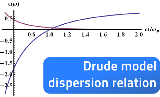
We now have also found the relative permittivity as
You can see an example plot of a Drude dispersion relation, i.e. \(\varepsilon\left(\omega\right)\), in the intro graphic right to the problem statement or below in the background section, where we also compare the model to some real experimental data.
Conductivity within the Drude Model
Generally, the Drude model is used to calculate the conductivity from Ohm's law. With the given solution of the equations of motion, it is quite easy to also derive this result.
First of all, we treat the electrons naturally as conductive current with the given electron density to find the current density:
Now, using Ohm's law, we find the conductivity
We can also see that \(\chi\left(\omega\right)=\mathrm{i}\sigma\left(\omega\right)/\omega\).
Of course, this is not a coincidence. Remember that we could (almost) entirely forget about the conductivity if we use the generalized permittivity
as we have derived in "The "Permittivity" of Graphene" from
with the use of Ohm's law.
Background: The Drude Model as a Working Horse in Theoretical Electrodynamics
Now we have derived the Drude model dispersion relation which was quite easy once we went into Fourier space. Now the main questions are, if such a dispersion relation can really reflect the electrodynamic properties of real metals and how this description may be useful.
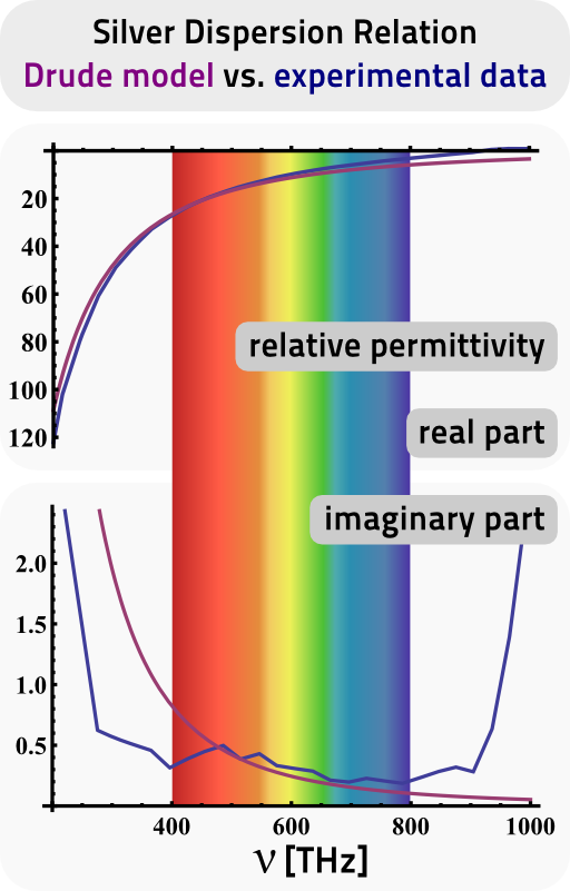
On the right you can see a comparison of the dispersion relation of silver taken from Johnson and Christy's "Optical Constants of the Noble Metals", Phys. Rev. B 6 (1972), pdf. What we can see is that we find a very good agreement of the data to a Drude model fit, both for real and imaginary part of the relative permittivity εr. Optical frequencies are decoded by their very colors.
The agreement to experimental data leads to a boiling down of the whole dispersion relation to just two parameters - plasma frequency ωp and loss rate γ.
Such a simple theoretical description is a huge advantage compared to numerical data: Researchers can rely on the dispersion relation and derive other theories on top of the Drude description.
This lead to a better understanding of certain metamaterial effects^ or of metal particles coupled to quantum systems^.. The Drude model is so widely applied that it is hard to find publications investigating light-metal-interactions that to not use it.
If you liked the simplicity of the Drude model, you can try to generalize it to the case when a magnetic field is present, see "The Dispersion Relation of a Magnetized Plasma". In this problem you will find that the magnetic field makes the response of the plasma strongly depends on the polarization of the electric field which will finally bring us to an understanding of the so-called Faraday rotation.


