The Faraday Rotation - How an Electron Gas and a Magnetic Field Rotate a Plane Wave

In The Dispersion Relation of a Magnetized Plasma we found that a magnetic field alters the dispersion relation differently for left and right polarized light passing through a plasma. But what about a linear polarized wave? The emerging effect is termed the "Faraday Rotation" and has numerous applications. Find out what we can learn about the cosmos and graphene using this effect.

Problem Statement

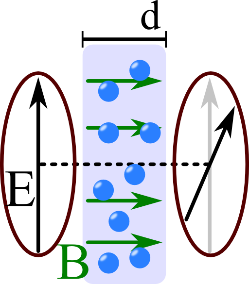
In the mentioned problem we assumed an electron density n_e and a constant magnetic field B = B₀·e_z.

We wanted to know the dispersion relation for circularly polarized light,

\[\mathbf{E}^{l/r}\left(\mathbf{r},t\right)    =    E_{0}\exp\left(\mathrm{i}\left(kz-\omega t\right)\right)\left[\mathbf{e}_{x}\pm\mathrm{i}\mathbf{e}_{y}\right]\ .\]

We found that

\[\epsilon_{r}^{l/r}\left(\omega\right)    =    1-\frac{\omega_{p}^{2}}{\omega\left(\omega\mp\Omega\right)}\]

with the plasma and cylcotron frequencies

\[\omega_{p}^{2}=\frac{n_{e}e^{2}}{\epsilon_{0}m_{e}}  ,   \Omega=eB_{0}/m_{e}\ .\]

In conclusion the response of the electron plasma was strongly depending on the polarization of the wave.

Find the rotation of a plane wave polarized in x direction passing through a magnetized plasma of thickness d  for frequencies much greater than both ω_p and Ω!

Hints

What is the relation of a circular and a linear polarized plane wave?

How can we know the rotation from the dispersion relation?

Solution

We know that a linear polarized plane wave can be seen as a superposition of circular polarized ones. From

\[\begin{eqnarray*}\mathbf{E}^{l/r}\left(\mathbf{r},t\right) & = & E_{0}\exp\left(\mathrm{i}\left(kz-\omega t\right)\right)\left[\mathbf{e}_{x}\pm\mathrm{i}\mathbf{e}_{y}\right]\end{eqnarray*}\]

we can see that

\[\begin{eqnarray*}\mathbf{E}^{x}\left(\mathbf{r},t\right) & = & \frac{1}{2}\left(\mathbf{E}^{l}\left(\mathbf{r},t\right)+\mathbf{E}^{r}\left(\mathbf{r},t\right)\right)\ .\end{eqnarray*}\]

Now we may treat the plasma as a medium with the derived dispersion relation. The dispersion relation is given by:

\[\begin{eqnarray*}k_{l,r}\left(\omega\right) & = & \sqrt{\epsilon_{r}^{l,r}\left(\omega\right)}k_{0}\ .\end{eqnarray*}\]

Since the high-frequency case is considered we may use a Taylor expansion of the relative permittivity. This will yield the difference between both polarizations. It is

\[\begin{eqnarray*}\sqrt{\epsilon_{r}^{l/r}\left(\omega\right)} & = & \sqrt{1-\frac{\omega_{p}^{2}}{\omega\left(\omega\mp\Omega\right)}}\\ & = & 1-\frac{\omega_{p}^{2}}{2\omega^{2}}\mp\frac{\omega_{p}^{2}\Omega}{2\omega^{3}}+\mathcal{O}\left(\omega^{-4}\right)\ . \end{eqnarray*}\]

Putting the latter result into the electric field we find an equation for the electric field inside the plasma:

\[\begin{eqnarray*}\mathbf{E}^{x}\left(\mathbf{r},t\right) & = & \frac{E_{0}}{2}\exp\left(-\mathrm{i}\omega t\right)\left(\exp\left(\mathrm{i}k_{l}z\right)\left[\mathbf{e}_{x}+\mathrm{i}\mathbf{e}_{y}\right]+\exp\left(\mathrm{i}k_{l}z\right)\left[\mathbf{e}_{x}-\mathrm{i}\mathbf{e}_{y}\right]\right)\\& = & \frac{E_{0}}{2}\exp\left[\mathrm{i}\left\{ \left(1-\frac{\omega_{p}^{2}}{2\omega^{2}}\right)k_{0}z-\omega t\right\} \right]\\& & \cdot\left(\exp\left({\color{red}-}\mathrm{i}\frac{\omega_{p}^{2}\Omega}{2\omega^{3}}k_{0}z\right)\left[\mathbf{e}_{x}+\mathrm{i}\mathbf{e}_{y}\right]+\exp\left({\color{red}+}\mathrm{i}\frac{\omega_{p}^{2}\Omega}{2\omega^{3}}k_{0}z\right)\left[\mathbf{e}_{x}-\mathrm{i}\mathbf{e}_{y}\right]\right)\ .\end{eqnarray*}\]

Now we can see that after a certain propagation distance d both polarizations have accumulated different phases. To find how much the incident wave has been rotated we just have to look for the prefactors in front of e_y, the calculation for e_x would be similar:

\[\begin{eqnarray*} \mathrm{i}\left(\exp\left(-\mathrm{i}\frac{\omega_{p}^{2}\Omega}{2\omega^{3}}k_{0}d\right)-\exp\left(+\mathrm{i}\frac{\omega_{p}^{2}\Omega}{2\omega^{3}}k_{0}d\right)\right)\mathbf{e}_{y} & = & 2\sin\left(\frac{\omega_{p}^{2}\Omega}{2\omega^{3}}k_{0}d\right)\mathbf{e}_{y}\ . \end{eqnarray*}\]

Hence we find a rotation of

\[\begin{eqnarray*} \varphi & = & \frac{\omega_{p}^{2}\Omega}{2\omega^{3}}k_{0}d\ . \end{eqnarray*}\]

For some applications for this effect please have a look at the following background!

 

---

Background: The Faraday Effect and its Applications

It is clear that any time more or less free charged particles are passed by an electromagnetic wave and a magnetic field is involved, one might observe the Faraday Effect we are about to calculate. One tool designed from the effect is the Faraday Rotator changing the angle of polarization due to the studied effect.

If one knows the rotation and the plasma density, one can in principle measure the magnetic field. This is also true for the biggest laboratory one can imagine - the universe! See for example Faraday Rotation of Microwave Background Polarization by a Primordial Magnetic Field on how the effect is used to unravel the last secrets of space and time.

We might very well change the length scales from lightyears to Ångström. Here we find the very promising material graphene which is a monolayer of carbon atoms. Graphene has an extremely high conductivity because of hybridized electrons. Thus, when a light wave is passing through this approximately five Ångström thick layer one might still expect a measurable Faraday Rotation. An experiment was done in 2010 and show the extraordinary properties of graphene, see Giant Faraday rotation in single- and multilayer graphene.