Tags: Dispersion Relation
![]() It is known that a free electron gas prone to a periodic electric field obeys oscillations. One might ask what happens if an additional external magnetic field is acting on the plasma. In this problem we will discover how the magnetic field changes the dispersion relation. This will later allow us to understand how the magnetic field in the universe is measured using the "Faraday Rotation".
It is known that a free electron gas prone to a periodic electric field obeys oscillations. One might ask what happens if an additional external magnetic field is acting on the plasma. In this problem we will discover how the magnetic field changes the dispersion relation. This will later allow us to understand how the magnetic field in the universe is measured using the "Faraday Rotation".
Problem Statement
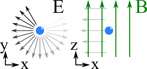
We want to assume an electron in a constant magnetic field parallel to the z axis, B = B0ez.
The free (non-interacting) electrons shall be driven by a left/right circularly polarized plane wave propagating in z-direction, see figure on the right:
Find the equations of motion for the electron. Use the assumptions that the range of the electron movement is much smaller than the wavelength and that its speed is much slower than the speed of light.
Solve the equations of motion to find the electron displacement.
Then, calculate the dispersion relation of the system assuming an electron density ne.
This problem is very helpful to understand "The Faraday Rotation - How an Electron Gas and a Magnetic Field Rotate a Plane Wave" and a generalization of the Drude model which describes the electrodynamic properties of metals.
Hints
Which force is responsible for the movement of a charged body in an electromagnetic field?
How is the electron displacement related to the polarization?
What is the connection between polarization and permittivity?
Ok, let's jump straight into the solution - there are a couple of calculations to be done!
Solution
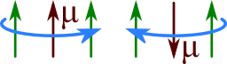
Before we go into details lets imagine what might be happening. We can already guess that a single electron will follow the movement of the electric field of the wave. That means, it will make a circular motion. Such a motion however implies a magnetic moment \(\boldsymbol{\mu}\) that will interact with the magnetic field \(\mathbf{}B\). \(\boldsymbol{\mu}\) and \(\mathbf{}B\) being parallel is an energetically favorable situation (left picture below) whereas the contrary holds for the antiparallel case (right picture). Now we have to figure out what this means in mathematical terms and how it is reflected in the dispersion relation.
We can divide our efforts into three steps. It is very useful to make the calculations in a complex notation. To do so, we first have to know howa circular polarized monochromatic wave is expressed in this way. Next we calculate the electron displacement using the Lorentz force.
At last we have to use our results to calculate the polarization and thus the relative permittivity.
Circular Polarized Light - Complex Notation
In real space, a right (left) circularly polarized plane may be defined by\[\begin{eqnarray*}\mathbf{E}^{r/l}\left(\mathbf{r},t\right) & = & E_{0}\left\{ \cos\left(kz-\omega t\right)\mathbf{e}_{x}\pm\sin\left(kz-\omega t\right)\mathbf{e}_{y}\right\} \ .\end{eqnarray*}\]Remark: This choice is basically convention. The one I used here should be the same as used in optics textbooks. It is based on the interpretation that a right-handed polarization is a clockwise rotation of the electric field in a spatially fixed plane viewing in the direction of the source. However, engineers use the opposite convention as defined in the "IEEE Standard Definition of Terms for Antennas".
Using \(\exp\left(\mathrm{i}x\right)=\cos x+\mathrm{i}\sin x\), we may write:\[\begin{eqnarray*} \mathbf{E}^{r/l}\left(\mathbf{r},t\right) & = & \frac{1}{2}E_{0}\Re\left\{ \exp\left(\mathrm{i}\left(kz-\omega t\right)\right)\mathbf{e}_{x}\mp\mathrm{i}\exp\left(\mathrm{i}\left(kz-\omega t\right)\right)\mathbf{e}_{y}\right\} \ .\\ & = & \frac{1}{2}E_{0}\Re\left\{ \exp\left(\mathrm{i}\left(kz-\omega t\right)\right)\left[\mathbf{e}_{x}\mp\mathrm{i}\mathbf{e}_{y}\right]\right\} \ . \end{eqnarray*}\]Hence, the part in brackets corresponds to circular polarized plane waves in the complex notation.
The Electron Displacement
The equations of motion are given due to the Lorentz force:\[\begin{eqnarray*} m_{e}\ddot{\mathbf{r}}_{l/r} & = & -e\left[\mathbf{E}\left(\mathbf{r},t\right)+\dot{\mathbf{r}}_{l/r}\times\mathbf{B}\left(\mathbf{r},t\right)\right]\\ & = & -e\left[E_{0}\exp\left(\mathrm{i}\left(kz-\omega t\right)\right)\left[\mathbf{e}_{x}\pm\mathrm{i}\mathbf{e}_{y}\right]+\dot{\mathbf{r}}_{l/r}\times B_{0}\mathbf{e}_{z}\right]\\ & \approx & -e\left[E_{0}\exp\left(-\mathrm{i}\omega t\right)\left[\mathbf{e}_{x}\pm\mathrm{i}\mathbf{e}_{y}\right]+\dot{\mathbf{r}}_{l/r}\times B_{0}\mathbf{e}_{z}\right]\ . \end{eqnarray*}\]We have used in the last step that \(kz\approx0\) because the electron motion shall be small compared to the wavelength. Furthermore, due to the assumed slow motion any relativistic effects are neglected since we just use the velocity here. Obviously the electron's motion can be studied in the x-y-plane since there is no force in \(z\) direction. The electric field obeys a \(\exp\left(-\mathrm{i}\omega t\right)\) dependency. Since further the magnetic field is constant, we can use an ansatz of the form\[\begin{eqnarray*} \mathbf{r}_{l/r}\left(t\right) & = & \mathbf{r}_{l/r,0}\exp\left(-\mathrm{i}\omega t\right) \end{eqnarray*}\]yielding\[\begin{eqnarray*} -m_{e}\omega^{2}\mathbf{r}_{l/r,0} & = & -e\left[E_{0}\left[\mathbf{e}_{x}\pm\mathrm{i}\mathbf{e}_{y}\right]-\mathrm{i}\omega B_{0}\mathbf{r}_{l/r,0}\times \mathbf{e}_{z}\right] \end{eqnarray*}\]where we have cancelled the time dependency in all factors. We can see that this equation only has a solution if \(\mathbf{r}_{l/r,0}=r_{l/r,0}\left(\mathbf{e}_{x}\pm\mathrm{i}\mathbf{e}_{y}\right)\).Using \(\left(\mathbf{e}_{x}\pm\mathrm{i}\mathbf{e}_{y}\right)\times\mathbf{e}_{z}=-\mathbf{e}_{y}\pm\mathrm{i}\mathbf{e}_{x}=\pm\mathrm{i}\left(\mathbf{e}_{x}\pm\mathrm{i}\mathbf{e}_{y}\right)\)we find\[\begin{eqnarray*}-m_{e}\omega^{2}r_{l/r,0} & = & -e\left[E_{0}\pm\omega B_{0}r_{l/r,0}\right]\ ,\\ r_{l/r} & = & \frac{eE_{0}}{m_{e}\omega^{2}\mp e\omega B_{0}}=\frac{eE_{0}}{m_{e}}\frac{1}{\omega\left(\omega\mp\Omega\right)} \end{eqnarray*}\]with the well-known (non-relativistic) cyclotron frequency \(\Omega=eB_{0}/m_{e}\). Note that using a monochromatic plane-wave is equivalent to a calculation in frequency space with only one frequency component. Thus, \(\omega\) is not only a parameter but rather a variable.
Next, we will use this result to calculate the dispersion relation.
Dispersion Relation
While analysing the movement of a free electron we implicitly implied a linear response to the driving electric field. Then, the electric displacement field is given by the relation\[\begin{eqnarray*} \mathbf{D}\left(\mathbf{r},\omega\right) & = & \epsilon_{0}\mathbf{E}\left(\mathbf{r},\omega\right)+\mathbf{P}\left(\mathbf{r},\omega\right)\\ & = & \epsilon_{0}\mathbf{E}\left(\mathbf{r},\omega\right)+\epsilon_{0}\chi\left(\mathbf{r},\omega\right)\mathbf{E}\left(\mathbf{r},\omega\right)\\ & = & \epsilon_{0}\epsilon_{r}\left(\mathbf{r},\omega\right)\mathbf{E}\left(\mathbf{r},\omega\right)\ . \end{eqnarray*}\]We have used the linear susceptibility \(\chi\left(\mathbf{r},\omega\right)\) and the relative permittivy \(\epsilon_{r}\left(\mathbf{r},\omega\right)\) to express the polarization \(\mathbf{P}\left(\mathbf{r},\omega\right)\) in terms of \(\mathbf{E}\left(\mathbf{r},\omega\right)\). Note that the latter equation does not make sense in a time representation. There, one has to consider the response of the medium which usually involves an integration over the past. In our case we know that the polarization is given by\[\begin{eqnarray*} p_{l/r}\left(\omega\right) & = & -er_{l/r}\left(\omega\right)\\ & = & -\frac{e^{2}E_{0}}{m_{e}}\frac{1}{\omega\left(\omega\mp\Omega\right)}\ .\end{eqnarray*}\]The latter equation is scalar since we keep in mind that this polarization holds with respect to left and right circular polarized light. However, a plasma containing only of one electron may be slightly underpopulated. For the overall polarization we have to incorporate an electron density \(n_{e}\). Then we can use the relation of \(\mathbf{P}\) and \(\mathbf{E}\) to finally arrive at the susceptibility \(\chi_{l/r}\). Again using scalar quantities we find\[\begin{eqnarray*} P_{l/r}\left(\omega\right) & = & -\frac{n_{e}e^{2}}{m_{e}}\frac{E_{0}}{\omega\left(\omega\mp\Omega\right)}\\ & = & \epsilon_{0}\chi_{l,r}\left(\omega\right) \left|E_{l/r}\left(\omega\right)\right|\ \text{, so}\\ \chi_{l,r}\left(\omega\right) & = & \frac{P_{l/r}\left(\omega\right)}{\epsilon_{0}\chi_{l,r}\left(\omega\right)E_{0}}\\ & = & -\frac{n_{e}e^{2}}{\epsilon_{0}m_{e}}\frac{1}{\omega\left(\omega\mp\Omega\right)}\ . \end{eqnarray*}\]Here, we discover the very important plasma frequency\[\begin{eqnarray*} \omega_{p}^{2} & = & \frac{n_{e}e^{2}}{\epsilon_{0}m_{e}} \end{eqnarray*}\]which is a characteristic quantity for free-electron oscillations.
Using the determined susceptibility we finally find the dispersion relation\[\begin{eqnarray*} \epsilon_{r}^{l/r}\left(\omega\right) & = & 1+\chi_{l/r}\left(\omega\right)\\ & = & 1-\frac{\omega_{p}^{2}}{\omega\left(\omega\mp\Omega\right)}\ . \end{eqnarray*}\]This dispersion relation only has two parameters: the plasma and cyclotron frequencies \(\omega_p\) and \(\Omega\), respectively. This makes it easy to understand its characteristics, see the figure below.
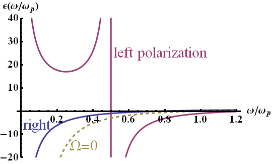
The dispersion relation of a magnetized plasma with respect to left and right polarized plane waves. Here a ratio of \(\Omega/\omega_p = 0.5\) has been chosen meaning a relatively high magnetic field. One can see that in the limit \(\omega\rightarrow\infty\) both solutions converge.
However for low energies one can see a clear distinction. Interestingly, the left polarization is highly dispersive for low frequencies and obeys a dielectric behavior for \(\omega < \Omega\). On the contrary, the right polarization acts like a metal. For comparison the dispersion without magnetic field is also shown.
I hope you found this dispersion relation of a magnetized plasma as interesting as I did! We have effectively shown how the plasma's optical properties can be tuned.


