Tags: Directivity / Poynting Vector / Dipole / Superposition Principle
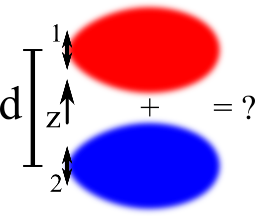
![]() The simplest form of an antenna array are two short dipole antennas. In this problem you will learn how a phase difference between the currents of both antennas affects their combined radiation pattern.
The simplest form of an antenna array are two short dipole antennas. In this problem you will learn how a phase difference between the currents of both antennas affects their combined radiation pattern.
Problem Statement
A single short dipole antenna with length L ≪ λ shall obey a current
\[\begin{eqnarray*} I\left(z,t\right)&=&\begin{cases} I_{0}e^{-\mathrm{i}\omega_{0}t}\left(1-2\frac{\left|z\right|}{L}\right) & \left|z\right|\leq L/2\\
0 & \mathrm{else} \end{cases}\ . \end{eqnarray*}\]
Calculate the dipole moment \(\mathbf{p}\left(t\right)\) of such a current and its radiated power.
Now, suppose that two of these antennas are placed along the z axis with a separation d.
Assume that there is an intrinsic phase difference between both currents, say \(I_{0,2}=I_{0,1}\exp\left(-\mathrm{i}\Delta\phi_{21}^{0}\right)\).
Then, what is the angular distribution of the radiated power \(dP/d\Omega\) in this case?
Discuss the qualitative behavior of \(dP/d\Omega\) for \(\Delta\phi_{21}^{0}=0\) and \(\pi/2\) with both \(d=\lambda\) and \(\lambda/2\).
Hint
Use your knowledge about the radiation of a single dipole and combine it with the superposition principle. But take care, do not simplify too much!
After the hint on superposition, let's find the solution for the radiation emitted by two dipole antennas!
We will first find out the power radiated by the given short dipole antenna. Using this result we will be able to find the radiation characteristic for two antennas with a certain distance and phase difference.
Single Dipole Antenna
To calculate the dipole moment of a source with one-dimensional current
\[\begin{eqnarray*} \mathbf{j}\left(\mathbf{r},t\right)=\delta\left(x,y\right)\cdot I\left(z,t\right)&=&\delta\left(x,y\right)\cdot\begin{cases}I_{0}e^{-\mathrm{i}\omega_{0}t}\left(1-2\frac{\left|z\right|}{L}\right) & \left|z\right|\leq L/2\\0 & \mathrm{else}\end{cases}\ , \end{eqnarray*}\]
we can employ the conservation law
\[\begin{eqnarray*} \nabla\cdot\mathbf{j}\left(\mathbf{r},t\right)+\partial_{t}\rho\left(\mathbf{r},t\right)&=&0\ :\\\partial_{t}\rho\left(x=0,y=0,z,t\right)&=&-\partial_{z}I\left(z,t\right)\\&=&\frac{2I_{0}}{L}e^{-\mathrm{i}\omega_{0}t}\cdot\begin{cases}-1 & z>0\\1 & z<0\end{cases}\ . \end{eqnarray*}\]
Please note that we disregard the discontinuity of the current at the termination of the antenna. This part would result in some delta-terms at the termination \(\propto z\left(1-2\left|z\right|/L\right)\delta\left(1-2\left|z\right|/L\right)\). These terms, however, will not have an effect for the calculation of the dipole moment so we might leave them out here.
Now we can solve the differential equation at hand on the z axis to find
\[\begin{eqnarray*} \rho\left(z,t\right)&=&\frac{2I_{0}}{-\mathrm{i}\omega_{0}L}e^{-\mathrm{i}\omega_{0}t}\cdot\begin{cases}-1 & z>0\\1 & z<0\end{cases}\ . \end{eqnarray*}\]
Since the antennas are made of metal, we may assume that the constant part vanishes, i.e. \(\rho\left(z,t=0\right)=0\).
Then, the dipole moment is given by
\[\begin{eqnarray*} \mathbf{p}&=&\int\mathbf{r}^{\prime}\rho\left(\mathbf{r}^{\prime},t\right)dV^{\prime}\\&=&\int\mathbf{r}^{\prime}\delta\left(x,y\right)\rho\left(z,t\right)dV^{\prime}\\&=&\int z^{\prime}\rho\left(z,t\right)dz^{\prime}\mathbf{e}_{z}\\&=&\frac{2I_{0}}{-\mathrm{i}\omega_{0}L}e^{-\mathrm{i}\omega_{0}t}\left\{ -\left[\frac{z^{2}}{2}\right]_{0}^{L/2}+\left[\frac{z^{2}}{2}\right]_{-L/2}^{0}\right\} \\&=&\frac{I_{0}L}{2\mathrm{i}\omega_{0}}e^{-\mathrm{i}\omega_{0}t}\ . \end{eqnarray*}\]
Note that for the averaging we have to take real quantities and integrate over an oscillation period. Here, we calculate
\[\begin{eqnarray*} \left\langle \mathbf{p}^{2}\right\rangle \sim\left\langle \sin^{2}\omega_{0}t\right\rangle &=&\frac{\omega_{0}}{2\pi}\int_{-\pi/\omega_{0}}^{\pi/\omega_{0}}\sin^{2}\left(\omega_{0}t\right)dt=\frac{1}{2} \ . \end{eqnarray*}\]
The radiated power is then given by
\[\begin{eqnarray*} P&=&\frac{\omega_{0}^{4}}{12\pi\varepsilon_{0}c^{3}}\left\langle \mathbf{p}^{2}\right\rangle =\frac{\omega_{0}^{4}}{12\pi\varepsilon_{0}c^{3}}\frac{1}{2}\frac{I_{0}^{2}L^{2}}{4\omega_{0}^{2}}\\&=&\frac{\omega_{0}^{2}I_{0}^{2}L^{2}}{96\pi\varepsilon_{0}c^{3}}\ . \end{eqnarray*}\]Furthermore,\[\begin{eqnarray*} \left\langle \mathbf{S}\right\rangle &=&\frac{\omega_{0}^{4}}{32\pi^{2}\varepsilon_{0}c^{3}}\frac{\left\langle \mathbf{p}^{2}\right\rangle \sin^{2}\theta}{r^{2}}\mathbf{e}_{r}\\&=&\frac{\omega_{0}^{4}}{32\pi^{2}\varepsilon_{0}c^{3}}\frac{1}{2}\frac{I_{0}^{2}L^{2}}{4\omega_{0}^{2}}\frac{\sin^{2}\theta}{r^{2}}\mathbf{e}_{r}\ ,\\\frac{dP}{d\Omega}&=&\frac{\omega_{0}^{2}I_{0}^{2}L^{2}}{256\pi^{2}\varepsilon_{0}c^{3}}\sin^{2}\theta\ . \end{eqnarray*}\]
We will use the angular distribution of radiated power later on.
Two Antennas: Effect of Separation and Phase Difference
Now that we know what one such short antenna does, we can figure out what happens if two of them are are forming an antenna array. To do this, we have to in principle look at their corresponding farfield distributions taking into account interference effects with respect to their distance \(d\). The reason why we cannot use the resulting dipole moment directly can be found at the bottom of the page.
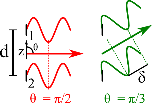 Luckily, we can solve this problem geometrically using the path difference depending on direction, see figure on the right. We find that the phase difference between both dipoles in the farfield is given by\[\begin{eqnarray*} \text{\delta}_{21}&=&-d\cos\theta\ . \end{eqnarray*}\]Note that we again take the mismatch from the second dipole antenna with respect to the first resulting in the minus sign. This mismatch corresponds to a phase difference between second and first antenna of \[\begin{eqnarray*} \Delta\phi_{21}^{\theta} &=& \frac{2\pi}{\lambda}\cdot\delta_{21}=-k\cdot d\cos\theta \end{eqnarray*}\]where we have introduced the wavenumber \(k=2\pi/\lambda\).
Hence, the overall phase difference yields for the fields
\[\begin{eqnarray*} \mathbf{E}_{2}\left(\mathbf{r},t\right)&=&\mathbf{E}_{1}\left(\mathbf{r},t\right)\exp\left\{ -\mathrm{i}\Delta\phi_{21}\right\} \ \mathrm{with}\\\Delta\phi_{21}&\equiv&\Delta\phi_{21}^{0}+k\cdot d\cos\theta\ . \end{eqnarray*}\]
So, the total field is given by the superposition principle as
\[\begin{eqnarray*} \mathbf{E}\left(\mathbf{r},t\right)&=&\mathbf{E}_{1}\left(\mathbf{r},t\right)+\mathbf{E}_{2}\left(\mathbf{r},t\right)\\&=&\mathbf{E}_{1}\left(\mathbf{r},t\right)\left[1+\exp\left\{ -\mathrm{i}\Delta\phi_{21}\right\} \right]\ . \end{eqnarray*}\]
Note again that this approach is correct in the farfield \(k\left|\mathbf{r}\right|\gg1\) where this geometrical interpretation makes sense.
We are searching the angular distribution of the radiated power. This means we have to find the radial part of the Poynting vector for the given superposition. Remembering that the angular distriputed power for a single dipole was given by
\[\begin{eqnarray*} \frac{dP}{d\Omega}_{\mathrm{dip}}&=&\frac{\omega_{0}^{2}I_{0}^{2}L^{2}}{256\pi^{2}\varepsilon_{0}c^{3}}\sin^{2}\theta\ , \end{eqnarray*}\]we can see that\[\begin{eqnarray*} \frac{dP}{d\Omega}&=&\frac{dP}{d\Omega}_{\mathrm{dip}}\cdot\left|1+\exp\left\{ -\mathrm{i}\Delta\phi_{21}\right\} \right|^{2}\ , \end{eqnarray*}\]
since the radiated power was calculated from the radial Poynting vector, so, effectively from the square of the electrical farfield. We calculate
\[\begin{eqnarray*} \left|1+\exp\left\{ -\mathrm{i}\Delta\phi_{21}\right\} \right|^{2}&=&\left(1+\exp\left\{ -\mathrm{i}\Delta\phi_{21}\right\} \right)\left(1+\exp\left\{ \mathrm{i}\Delta\phi_{21}\right\} \right)\\&=&2\left(1+\cos\left(\Delta\phi_{21}\right)\right)\\&=&4\cos^{2}\left(\frac{\Delta\phi_{21}}{2}\right)\ , \end{eqnarray*}\]
where we have used and additional theorem for the cosine its property to be an even function. Note that for \(\Delta\phi_{21}=\pi\) and \(d=0\), hence currents with opposite sign and vitually overlapping dipoles, there is no radiation. So,
\[\begin{eqnarray*} \frac{dP}{d\Omega}&=&\frac{\omega_{0}^{2}I_{0}^{2}L^{2}}{64\pi^{2}\varepsilon_{0}c^{3}}\sin^{2}\theta\cos^{2}\left(\frac{\Delta\phi_{21}^{0}}{2}+\frac{k\cdot d}{2}\cos\theta\right)\ . \end{eqnarray*}\]
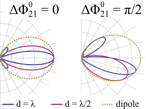
Now this formula is rather involved and we want to check the radiation behavior for some values of interesting phase differences. First of all, we let both currents in the antennas oscillate without phase difference, i.e. \(\Delta\phi_{21}^{0}=0\). What we expect is a dipole-like pattern with a however narrower lobe since we made the antenna effectively larger. For a separation as large as \(\lambda\) we further expect the occurrence of sidelobes, i.e. a radiation to higher angles but also an increase in the directivity (see again The Directivity of a Parabolic Reflector).
Furthermore, the radiation should obey a mirror symmetry with respect to the \(z\) axis since both antennas are equal as can be seen in the left part of the figure below. If we impose a phase difference \(\Delta\phi_{21}^{0}=\pi/2\), we find that upper and lower halfspace are no longer equivalent. Now, the lower hemisphere is favored by the radiation as can be seen in the right part of the figure. Note that a sign change in the phase difference leads to a strong emission into the upper hemisphere, respectively.
Generally we can state that a larger antenna results in more lobes but also higher directivity. Changing the phase of each element in an antenna consisting of dipoles leads to a tuning of the emission direction.
Why we cannot use the dipole moments directly
We could have thought that the question can be simply answered by a superposition of two dipoles and that we can calculate the radiated power from the resulting dipole moment. Although physical, this approach is not correct. From a short calculation of the dipole moments of each antenna,
\[\begin{eqnarray*} \mathbf{p}_{1,2}&=&\int z^{\prime}\rho\left(z^{\prime}\mp d/2\right)e^{\pm\mathrm{i}\Delta\phi/2}dz\mathbf{e}_{z}\\&=&e^{\pm\mathrm{i}\Delta\phi/2}\int\left(z^{\prime}\pm d/2\right)\rho\left(z^{\prime}\right)dz\mathbf{e}_{z}\\&=&e^{\pm\mathrm{i}\Delta\phi/2}\int z^{\prime}\rho\left(z^{\prime}\right)dz\mathbf{e}_{z}\\&=&e^{\pm\mathrm{i}\Delta\phi/2}\mathbf{p}\ , \end{eqnarray*}\]
we can see that in our case the dipole moment is invariant under translations; the phase is just corresponding to our assumption. We have used in the last step that the integrated charge over each antenna vanishes. So, if both antennas are out of phase by \(\Delta\phi=\pi\), there should be no radiation at all in this simple picture, since
\[\begin{eqnarray*} \mathbf{p}_{1}+\mathbf{p}_{2}&=&\left(e^{\mathrm{i}\pi/2}+e^{-\mathrm{i}\pi/2}\right)\mathbf{p}=0\ . \end{eqnarray*}\]
Such an approach can be falsified e.g. by two distant dipole sources which will for sure radiate. So, why is this approach not correct?
To calculate the power radiated by a dipole we are integrating the time-averaged radial part of the Poynting vector \(\left\langle \mathbf{S}\left(\mathbf{r},t\right)\right\rangle =\left\langle \mathbf{E}\left(\mathbf{r},t\right)\times\mathbf{H}\left(\mathbf{r},t\right)\right\rangle\).
So, since \(\mathbf{H}\propto\mathbf{E}\) in the farfield, we have to look at the electric field itself. Otherwise, we lose any information about interference!
Background: Radiation of a Dipole
The time-averaged radiated power of a dipole with dipole moment \(\mathbf{p}\) oscillating at some angular frequency \(\omega_{0}\) is given by
\[\begin{eqnarray*} P&=&\frac{\omega_{0}^{4}}{12\pi\varepsilon_{0}c^{3}}\left\langle \mathbf{p}^{2}\right\rangle \ . \end{eqnarray*}\]This relation can be calculated from the time-averaged Poynting vector of such a source in the farfield,\[\begin{eqnarray*} \left\langle \mathbf{S}\right\rangle &=&\frac{\omega_{0}^{4}}{32\pi^{2}\varepsilon_{0}c^{3}}\frac{\left\langle \mathbf{p}^{2}\right\rangle \sin^{2}\theta}{r^{2}}\mathbf{e}_{r}\equiv\frac{1}{r^{2}}\frac{dP}{d\Omega}\mathbf{e}_{r}\ , \end{eqnarray*}\]
where \(\theta\in\left[0,\pi\right]\) is the angle between \(\mathbf{p}\) and a vector at the position of (thought) measurement. If \(\mathbf{p}\) is along the \(z\) axis, this angle is the usual polar angle in spherical coordinates.
The quantity \(dP/d\Omega\) is usually termed the angular distribution of the radiated power and goes characteristically with \(\sin^{2}\theta\) for a dipole. Note that as usual \(d\Omega=\sin\theta d\theta d\varphi\).


