In this problem you will learn how to apply the Fourier Transformation to a simple exponentially decaying electric field. We will see the definitions applied and some nice physics unfolds!
Problem Statement
To get the frequency-spectrum of an electric field we use the so-called Fourier-Transformation. Calculate the spectrum of the following pulse:
\[f(t)=te^{-\alpha\left|t\right|},\alpha>0\]
Hint
Separate the integral in two parts for \(t<0\) and \(t>0\) and use integration by parts.
Solution
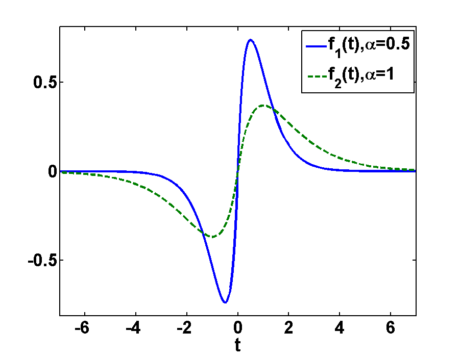
Fig.1 shows the the function \(f(t)\) for two different damping constants \(\alpha>0\). In order to get its Fourier spectrum we will straight forwardly apply the Fourier transformation on \(f(t)\), considering the different signs of \(t\) in order to get \(f(\omega)\) as a function of the frequency \(\omega\).
\begin{eqnarray*}FT\left[{f(t)}\right](\omega)&=&\frac{1}{2\pi}\int\limits _{-\infty}^{\infty}{dt}\left({te^{-\alpha\left|t\right|}e^{i\omega t}}\right)\\&=&\frac{1}{2\pi}\int\limits _{-\infty}^{0}{dt}\left({te^{-\alpha\left|t\right|}e^{i\omega t}}\right)+\frac{1}{2\pi}\int\limits _{0}^{\infty}{dt}\left({te^{-\alpha\left|t\right|}e^{i\omega t}}\right)\\&=&\frac{1}{2\pi}\int\limits _{0}^{\infty}{dt}\left\{ -te^{-\alpha t}e^{-i\omega t}+te^{-\alpha t}e^{i\omega t}\right\} \\&=&\frac{1}{2\pi}\int\limits _{0}^{\infty}{dt}\left\{ t\left[e^{-(\alpha-i\omega)t}-e^{-(\alpha+i\omega)t}\right]\right\} \end{eqnarray*}
Using integration by parts for the integral in the last line
\[\int{u'v}=uv-\int{uv'}\]
we get
\begin{eqnarray*}2\pi FT\left[{f(t)}\right](\omega)&=&\int\limits_{0}^{\infty}{dt}\left(\underbrace{t}_{v}\left[\underbrace{e^{-(\alpha-i\omega)t}-e^{-(\alpha+i\omega)t}}_{u\prime}\right]\right)\\&=&\underbrace{\left.\left(-\frac{e^{-(\alpha-i\omega)t}}{\alpha-i\omega}+\frac{e^{-(\alpha+i\omega)t}}{\alpha+i\omega}\right)t\right|_{0}^{\infty}}_{0}+\int\limits _{0}^{\infty}{dt}\left(\frac{e^{-(\alpha-i\omega)t}}{\alpha-i\omega}-\frac{e^{-(\alpha+i\omega)t}}{\alpha+i\omega}\right)\\&=&-\left.\frac{e^{-(\alpha-i\omega)t}}{(\alpha-i\omega)^{2}}\right|_{0}^{\infty}+\left.\frac{e^{-(\alpha+i\omega)t}}{(\alpha+i\omega)^{2}}\right|_{0}^{\infty}=\frac{1}{(\alpha-i\omega)^{2}}-\frac{1}{(\alpha+i\omega)^{2}}\\&=&\frac{(\alpha+i\omega)^{2}}{(\alpha^{2}+\omega^{2})^{2}}-\frac{(\alpha-i\omega)^{2}}{(\alpha^{2}+\omega^{2})^{2}}=\frac{4i\omega\alpha}{\left(\alpha^{2}\omega^{2}\right)^{2}} \end{eqnarray*}
Hence, we get:
\begin{eqnarray*}FT\left[{f(t)}\right](\omega)=\frac{2i\alpha\omega}{\pi\left(\omega^{2}+\alpha^{2}\right)^{2}} \end{eqnarray*}
This result is illustrated in Fig.2 for different damping constants \(\alpha>0\). As we see, the real part of both functions \(f(\omega)\) vanishes, since \(f(t)\) is an odd function. Comparing \(f(t)\) with \(f(\omega)\) we see, that \(f(\omega)\) is more narrow than \(f(t)\). Otherwise the functions look quite similar.
Furthermore we see, that as expected the amplitude of the function depends on the damping factor. The amplitude decreases with stronger damping. It is also interesting to note that the broader function, \(\alpha = 0.5\), is now much more narrow. This is a general dualism between Fourier and real space: broad features get narrow and vice versa. Or, in other words, a very short pulse has a very broad frequency spectrum.
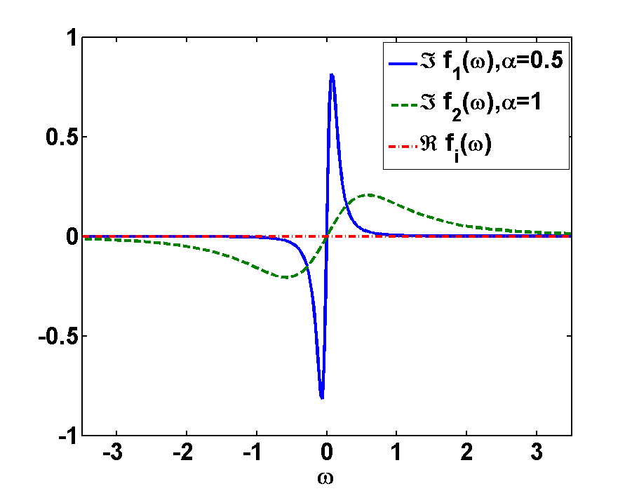 Fig2. - Illustration of the function \(f(\omega)\) for different damping factors \(\alpha>0\)