Tags: Dipole / Equations of Motion
Problem Statement
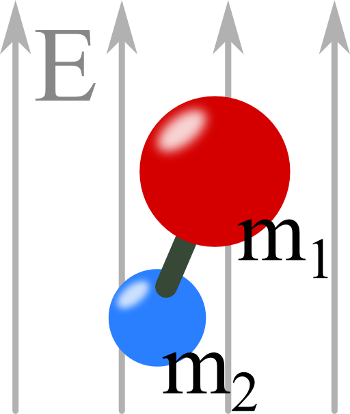
We want to assume that both charges are equal (no net charge). Furthermore they shall be separated by a fixed distance R and have two not necessarily equal masses m1 and m2.
Now there is a constant electrical field which may be parallel to the z-axis.
What happens to the molecule in the field? Describe its movement qualitatively!
You may want to proceed as follows:
- find the potential energy of the molecule in the electric field,
- determine conserved quantities using the Lagrange function and
- discuss the movement in terms of this conserved quantity.
Hints
The potential energy of a charge density ρ(r) in an external electrostatic potential ϕext(r) is given by
\[ \begin{eqnarray}V = \int \rho\left(\mathbf{r}\right) \phi_{\mathrm{ext}}\left(\mathbf{r}\right) dV\ . \end{eqnarray}\]
How can we use this hint to find the movement of a dipole in a constant electric field?
To understand the movement of the molecule we have to understand different aspects. First we have to find out how the molecule interacts with the external field.
Then, we use the Lagrange function to determine the conserved quantities. At last we will use these quantities to fully explore the movement. Enjoy!
Solution
First, we have to find the potential of the molecule in the electric field.
To achieve this, we use a Taylor expansion of the potential \(\phi_{\mathrm{ext}}\left(\mathbf{r}\right)\) inside the potential energy of a charge distribution \(\rho\left(\mathbf{r}\right)\):
\[\begin{eqnarray*}V &=& \int \rho\left(\mathbf{r}\right) \phi_{\mathrm{ext}}\left(\mathbf{r}\right) dV \\&=& \int \rho\left(\mathbf{r}\right)\left\{\phi_{\mathrm{ext}}\left(0\right) + \partial_i \phi_{\mathrm{ext}}\left(0\right)x^i + \frac{1}{2}\partial_{ij} \phi_{\mathrm{ext}}\left(0\right)x^i x^j\right\}dV\end{eqnarray*}\]
All terms in \(\phi_{\mathrm{ext}}\) are now constants and can be pulled out of the integral.
For our case,
\[\begin{eqnarray*}\rho\left(\mathbf{r}\right) &=& q\left[\delta(\mathbf{r}-\mathbf{r}_{1})-\delta(\mathbf{r}-\mathbf{r}_{2})\right]\end{eqnarray*}\]
and the only nonvanishing contribution comes from second term in the expansion:
\[\begin{eqnarray*}V&=&\nabla\phi_{\mathrm{ext}}\left(0\right)\cdot\int\rho\left(\mathbf{r}\right)\mathbf{r}dV\\&=&-q\mathbf{E}_{\mathrm{ext}}\left(0\right)\cdot\int q\left[\delta(\mathbf{r}-\mathbf{r}_{1})-\delta(\mathbf{r}-\mathbf{r}_{2})\right]\mathbf{r}dV\\&=&-q\mathbf{E}_{\mathrm{ext}}\left(0\right)\cdot\left(\mathbf{r}_{1}-\mathbf{r}_{2}\right)
\end{eqnarray*}\ .\]
The electric field is oriented along the \(z\) axis. Thus we are able express the latter result in terms of the angle \(\theta\).
This coordinate now coincides with the angle in between the electric field and the connection axis of the charges. Since the absolute value of \(\mathbf{r}_1-\mathbf{r}_2\) is fixed to \(R\), we find the potential energy
\[\begin{eqnarray*}V(\theta)&=&-qRE_{0}\cos\theta \end{eqnarray*}\]
which is just a certain form of the dipole coupling \(V_\mathrm{d} = -\mathbf{p}\cdot\mathbf{E}\).
Conserved Quantities
To find conserved quantities of the molecular motion it is very useful to use the Euler-Lagrange equations of motion. Having determined the potential energy, the Lagrange function is given by
\[\begin{eqnarray*}L &=& T - V \\ &=& \frac{m_{1}}{2}\dot{\mathbf{r}}_{1}^{2}+\frac{m_{2}}{2}\dot{\mathbf{r}}_{2}^{2}+qRE_{0}\cos\theta \ .\end{eqnarray*}\]
Naturally we express L in the centre-of-mass frame using
\[\begin{eqnarray*} \mathbf{r}& =& \mathbf{r}_2 -\mathbf{r}_2\quad \text{and the reduced mass}\\ m&=&\frac{m_1 m_2}{m_1 + m_2}\end{eqnarray*}\]
to obtain
\[\begin{eqnarray*}L&=&\frac{m}{2}\dot{\mathbf{r}}^{2}+qRE_{0}\cos\theta\end{eqnarray*}\ .\]
With just a little fantasy we can see that \(\mathbf{r} = R\mathbf{e}_r\) because of our choice of the coordinate system.
So, we might be able to express the Lagrange function in spherical coordinates just with respect to the angles \(\theta\) and \(\varphi\).
To achieve this, we need the time derivative of \(\mathbf{r}\) in spherical coordinates:
\[ \begin{eqnarray*}\dot{\mathbf{r}}&=&R\dot{\theta}\mathbf{e}_{\theta}+R\sin\theta\dot{\varphi}\mathbf{e}_{\varphi}\ . \end{eqnarray*} \]
Now we can finally express the Lagrange function in spherical coordinates:
\[\begin{eqnarray*}L&=&\frac{mR^{2}}{2}\left(\dot{\theta}^{2}+\sin^{2}\theta\dot{\varphi}^{2}\right)+qRE_0\cos\theta \ . \end{eqnarray*}\]
We are now also able to identify the conserved quantities of the system. First of all, the Lagrange function does not directly depend on time. Hence, the energy of the molecular motion is constant.
In addition we can also see that \(L\) does not depend on the angle \(\varphi\) directly. This implies conservation of the angular momentum
\[\begin{eqnarray*}p_{\varphi}=\frac{\partial L}{\partial\dot{\varphi}} &=& mR^{2}\sin^{2}\theta\dot{\varphi}\end{eqnarray*}\ .\]
The conserved quantities will help us understand the movement of the molecule in the following.
The overall movement of the molecule
The angle \(\theta\) has two meanings in our inertial frame. It is both coordinate and angle of the molecular axis to the electric field. Using the expression for the conserved angular momentum \(p_{\varphi}\), we find a relation between the angular velocity \(\dot{\varphi}\) and the angle \(\theta\):
\[\begin{eqnarray*}\dot{\varphi} & = & \frac{p_{\varphi}}{mR^{2}\sin^{2}\theta}\end{eqnarray*}\]
Note that neither \(\theta\) nor \(\dot{\varphi}\) is constant in general!
So, how can we employ this relationship to understand the movement? We may replace \(\dot{\varphi}\) entirely with terms in \(\theta\).
Next we can use the second conserved quantity, namely the energy \(\mathrm{E}\). Remembering that \(\mathrm{E}=T+V\) we find
\[\begin{eqnarray*}\mathrm{E} & = & \frac{mR^{2}}{2}\left(\dot{\theta}^{2}+\sin^{2}\theta\dot{\varphi}^{2}\right)-qRE_{0}\cos\theta\\& = & \frac{mR^{2}}{2}\left(\dot{\theta}^{2}+\frac{p_{\varphi}^{2}}{m^{2}R^{4}\sin^{2}\theta}\right)-qRE_{0}\cos\theta\ .\end{eqnarray*}\]
Now this formula is extremely useful. Using it we can entirely understand the movement of the molecule. Let us for example set \(p_{\varphi}=0\) for the moment. We find that \(\dot{\varphi}=0\) and
\[\begin{eqnarray*}\mathrm{E}\left(p_{\varphi}=0\right) & = & \frac{mR^{2}}{2}\dot{\theta}^{2}-qRE_{0}\cos\theta
\end{eqnarray*}\]
which is an oscillator equation for small \(\theta\). So, for small energies the molecule oscillates back and forth in \(\theta\).
But what about a non-vanishing angular momentum \(p_{\varphi}\neq0\)? Here one can look at the "effective potential''. This concept originates from celestial mechanics.
There, one is for example regarding the orbital motion of two bodies under the mutual influence of gravitation. If this motion has a certain angular momentum, the bodies may never collide.
In our case, the situation is just like that. Rearranging terms we find
\[\begin{eqnarray*}\frac{mR^{2}}{2}\dot{\theta}^{2} & = & \mathrm{E}-\frac{p_{\varphi}^{2}}{2mR^{2}\sin^{2}\theta}+qRE_{0}\cos\theta\\& \equiv & \mathrm{E}-V_{\mathrm{eff}}\left(\theta\right)\ .\end{eqnarray*}\]
Let us take some characteristic quantities for molecular systems to look at \(V_{\mathrm{eff}}\):
- \(p_{\varphi}=\hbar=6.63\times10^{-34}\text{Js}\) (Planck constant),
- \(m=m_{p}=1.67\times10^{-27}\text{kg}\) (proton mass),
- \(R=a_{0}=5.29\times10^{-10}\text{m}\) (Bohr radius) and
- \(q=e=1.60\times10^{-19}\text{C}\) (elementary charge).
Then,
\[\begin{eqnarray*}V_{\mathrm{eff}}\left(\theta\right) & = & \frac{\hbar^{2}}{2m_{p}a_{0}^{2}\sin^{2}\theta}-ea_{0}E_{0}\cos\theta\\& \approx & \frac{1.19\times10^{-21}\text{J}}{\sin^{2}\theta}-8.48\times10^{-30}\text{A s m}\cdot E_{0}\cos\theta\end{eqnarray*}\]
and we can see that an electric field has to be as big as \(10^{9\dots10} \text{V/m}\) to actually have an effect!
In the figure below you can see how \(V_{\mathrm{eff}}\) changes for different \(E_{0}\) from \(10^{10}\text{V/m}\) (blue curve) to \(6\times10^{10}\text{V/m}\) (green).
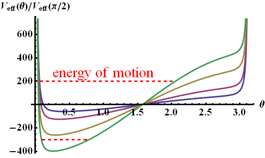
At different energies \(\mathrm{E}\) the molecule oscillates in a larger \(\theta\)-range. But similarly to the case of orbital motion, the points at \(\theta=0\) or \(\pi\) are never reached since \(p_{\varphi}\neq0\). Along with the angular movement in \(\varphi\), we can conclude that the molecule is performing a kind of precession.
We have seen that the details of the motion depend on the balance between the conserved quantities and the strength of the applied electric field.
Background: Symmetries and Conserved Quantities
The Lagrange function \(L\left(q_k,\dot{q}_k,t\right)\) is given in terms of generalized coordinates \(q_k\) and velocities \(\dot{q}_k\).
Conserved quantities are related to symmetries of the Lagrange function. If for some \(l\)
\[ \begin{eqnarray}\frac{\partial L\left(q_{k},\dot{q}_{k},t\right)}{\partial q_{l}}&=&0 \ , \mathrm{then}\quad p_l \equiv \frac{\partial L\left(q_{k},\dot{q}_{k},t\right)}{\partial\dot{q}_{l}}\end{eqnarray}\]
is a conserved quantity.
Do you remember why, regarding the Euler-Lagrange equation?