Tags: Rotational Symmetry / Cylindrical Coordinates / Ampere's law / Stoke's theorem / Biot-Savart's law
![]() We will directly use the Biot-Savart law to calculate the magnetic field of a thin wire via integration. The problem shall provide us with some intuition of Biot-Savart which we will also derive.
We will directly use the Biot-Savart law to calculate the magnetic field of a thin wire via integration. The problem shall provide us with some intuition of Biot-Savart which we will also derive.
Problem Statement
 In The Magnetic Field of an Infinite Wire we discussed the field of a not necessarily thin wire with a constant current j0ez.
We also discussed generalizations j0 → j(ρ). We made our calculations directly from the differential form of Ampère's law. If we assume a very thin wire, i.e. a current of the form
\[\mathbf{j}\left(\mathbf{r}\right) = I\delta\left(\rho\right)\mathbf{e}_{z}\]
in cylindrical coordinates, we may also calculate the magnetic field by direct integration via Biot-Savart's law,
\[\mathbf{B}\left(\mathbf{r}\right) = \frac{\mu_{0}I}{4\pi}\int\frac{d\mathbf{s}\times\left(\mathbf{r}-\mathbf{r}\left(s\right)\right)}{\left|\mathbf{r}-\mathbf{r}\left(s\right)\right|^{3}}\ ,\]
where the integral is over the curve of the thin wire.
- Calculate the magnetic field B(r) for the thin wire, infinitely extended in z using the Biot-Savart law.
- Extra: Derive the Biot-Savart law from the connection of the vector potential to the current.
Hints
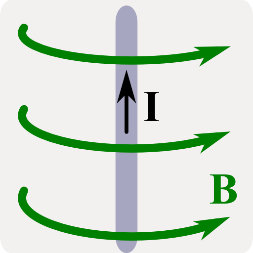
Even though the magnetic field of the infinite thin wire is a standard problem, draw a schematic. You got to make sure that you understand the symmetries in the system before you tackle the equations!
Remember that from the Poisson equation / inhomogeneous Laplace equation,
\[\Delta\mathbf{A}\left(\mathbf{r}\right)=-\mu_{0}\mathbf{j}\left(\mathbf{r}\right)\]
the vector potential is given by
\[\mathbf{A}\left(\mathbf{r}\right) = \frac{\mu_{0}}{4\pi}\int\frac{\mathbf{j}\left(\mathbf{r}^{\prime}\right)}{\left|\mathbf{r}-\mathbf{r}^{\prime}\right|}dV^{\prime}\ ,\]
just as in electrostatics for the electrostatic potential ϕ(r).
Using the electrostatics hint, we can turn over to magnetostatics again. Let's find the magnetic field of a thin wire!
Since we are quite thorough, we shall convince ourselves first that Biot-Savart's law is indeed correct. After that we will use it to determine the field of the thin wire.
Derivation of the Biot-Savart Law
There exist lots of different derivations of the Biot-Savart law. A lot of them use relations of differential elements ds causing differential magnetic fields dB(r). Let us try here an approach inspired by a proper curve parametrization r(s).
We start at the well-known relation of the vector potential to the current density:
\[\mathbf{A}\left(\mathbf{r}\right) = \frac{\mu_{0}}{4\pi}\int\frac{\mathbf{j}\left(\mathbf{r}^{\prime}\right)}{\left|\mathbf{r}-\mathbf{r}^{\prime}\right|}dV^{\prime}\]
For thin wires, we can explain j(r) as an integral over the positions r(s) of the wire,
\[\begin{eqnarray*} \mathbf{j}\left(\mathbf{r}\right)&=&I\,\int\frac{\partial\mathbf{r}\left(s\right)}{\partial s}/\left|\frac{\partial\mathbf{r}\left(s\right)}{\partial s}\right|\delta\left(\mathbf{r}-\mathbf{r}\left(s\right)\right)ds\\&=&I\,\int\mathbf{T}\left(s\right)\delta\left(\mathbf{r}-\mathbf{r}\left(s\right)\right)ds\ . \end{eqnarray*}\]
Here, T(s) is the normalized tangential vector. Then we find for the vector potential
\[\begin{eqnarray*} \mathbf{A}\left(\mathbf{r}\right)&=&\frac{\mu_{0}I}{4\pi}\int\frac{\mathbf{T}\left(s\right)\delta\left(\mathbf{r}^{\prime}-\mathbf{r}\left(s\right)\right)}{\left|\mathbf{r}-\mathbf{r}^{\prime}\right|}dV^{\prime}ds\\&=&\frac{\mu_{0}I}{4\pi}\int\frac{d\mathbf{s}}{\left|\mathbf{r}-\mathbf{r}\left(s\right)\right|}\ , \end{eqnarray*}\]
since we can change the order of integration and T(s)ds = ds is basically the definition of a curve integration.
Now we are almost ready. We just have to take the curl of the vector potential to find the magnetic field:
\[\begin{eqnarray*} \mathbf{B}\left(\mathbf{r}\right)=\nabla\times\mathbf{A}\left(\mathbf{r}\right)&=&\frac{\mu_{0}I}{4\pi}\int\nabla\times\frac{d\mathbf{s}}{\left|\mathbf{r}-\mathbf{r}\left(s\right)\right|}\ ,\\\nabla\times\frac{d\mathbf{s}}{\left|\mathbf{r}-\mathbf{r}\left(s\right)\right|}&=&\frac{1}{\left|\mathbf{r}-\mathbf{r}\left(s\right)\right|}\left(\nabla\times d\mathbf{s}\right)-d\mathbf{s}\times\nabla\frac{1}{\left|\mathbf{r}-\mathbf{r}\left(s\right)\right|}\\&=&+d\mathbf{s}\times\frac{\mathbf{r}-\mathbf{r}\left(s\right)}{\left|\mathbf{r}-\mathbf{r}\left(s\right)\right|^{3}}\ . \end{eqnarray*}\]
This leaves us in the end with the well-known Biot-Savart law:
\[\mathbf{B}\left(\mathbf{r}\right) = \frac{\mu_{0}I}{4\pi}\int\frac{d\mathbf{s}\times\left(\mathbf{r}-\mathbf{r}\left(s\right)\right)}{\left|\mathbf{r}-\mathbf{r}\left(s\right)\right|^{3}}\ .\]
Now let us apply our finding!
The Magnetic Field of the Thin Wire
For the thin and infinitely long wire we may very well parametrize the wire as r(s) = sez, s ∈ (-∞,∞).
In case fo the thin current wire, the Biot-Savart integration takes the form
\[\mathbf{B}\left(\mathbf{r}\right) = \frac{\mu_{0}I}{4\pi}\int\frac{\mathbf{e}_{z}\times\left(\mathbf{r}-s\mathbf{e}_{z}\right)}{\left|\mathbf{r}-s\mathbf{e}_{z}\right|^{3}}ds\ .\]
Now, the term \(\mathbf{e}_{z}\times s\mathbf{e}_{z}\) vanishes and we have to think what \(\mathbf{r}\) actually means.
Without any restriction we may say that \(\mathbf{r}=\rho\mathbf{e}_{\rho}\), thus somewhere in the x-y-plane: Because of the obvious translational symmetry of the current distribution in z direction and the rotational symmetry in φ direction, the field must obey the same symmetries. Then,
\[\begin{eqnarray*} \mathbf{B}\left(\rho\mathbf{e}_{\rho}\right)&=&\frac{\mu_{0}I}{4\pi}\int\frac{\mathbf{e}_{z}\times\rho\mathbf{e}_{\rho}}{\left|\rho\mathbf{e}_{\rho}-s\mathbf{e}_{z}\right|^{3}}ds\\&=&\frac{\mu_{0}I}{4\pi}\mathbf{e}_{\varphi}\int\frac{\rho}{\left(\rho^{2}+s^{2}\right)^{3/2}}ds\ . \end{eqnarray*}\]
This is a standard integral and we may solve it with the standard substitution
\[\begin{eqnarray*} \tan\alpha&=&s/\rho\ \text{, then}\\ds&=&\rho\frac{d\alpha}{\cos^{2}\alpha}\ \text{and}\\\mathbf{B}\left(\rho\mathbf{e}_{\rho}\right)&=&\frac{\mu_{0}I}{4\pi}\mathbf{e}_{\varphi}\int_{-\pi/2}^{\pi/2}\frac{\rho}{\rho^{3}\left(1+\tan^{2}\alpha\right)^{3/2}}\frac{\rho}{\cos^{2}\alpha}d\alpha\\&=&\frac{\mu_{0}I}{4\pi\rho}\mathbf{e}_{\varphi}\int_{-\pi/2}^{\pi/2}\cos\alpha d\alpha\ . \end{eqnarray*}\]
The last integral equals to 2. Then, since the solution cannot depend on the z position as we have discussed before, we find the magnetic field of the thin and infinitely long wire to be
\[\mathbf{B}\left(\mathbf{r}\right) = \frac{\mu_{0}I}{2\pi\rho}\mathbf{e}_{\varphi}\ .\]
This is of course exactly the result we already calculated for a not necessarily thin wire with net current I.
This does not surprise us from our experience in electrostatics. There, the field of spherically symmetric charge distributions is that of a point charge outside of the charge distribution. Here, we may find a corresponding principle.
Let us integrate Ampère's law over a certain surface A including all of the current density. Then, we find
\[\begin{eqnarray*} \int_{A}\nabla\times\mathbf{B}\left(\mathbf{r}\right)d\mathbf{A}&=&\int_{\partial A}\mathbf{B}\left(\mathbf{r}\right)d\mathbf{r}\\&=&\int_{A}\mu_{0}\mathbf{j}\left(\mathbf{r}\right)d\mathbf{A}\equiv I \end{eqnarray*}\]
using Stoke's law. So the magnetic field on a closed loop only depends on the current through the area of that loop.
At the end of the day we were able to find the magnetic field of a thin infinite wire with some mathematical effort. We needed to understand the Biot-Savart law and curve parametrization. Afterwards we were doing some standard tricks on the emerging integrals. However, if we would not have understood the symmetries of the system in the first place, this problem could be quite complicated, because we would run out of tricks for the integrals. As always, such tasks can be hugely simplified if only a coordinated system is chosen that is in line with the given symmetries.


