Tags: Telegrapher's equation / Reflection Coefficient / Impedance Matching
![]() For technical applications it is extremely important to be able to transfer as much energy from a transmission line to some load. In this problem we will learn how this is achieved and understand the basic principles signal reflection and impedance matching.
For technical applications it is extremely important to be able to transfer as much energy from a transmission line to some load. In this problem we will learn how this is achieved and understand the basic principles signal reflection and impedance matching.
Problem Statement
Find out how to impedance-match a serial oscillator circuit to a transmission line! Proceed as follows:
In The Transmission Line - Deriving the Telegrapher Equation we found that a transmission line is described by the telegrapher's equation
\[\begin{eqnarray*} \partial_{xx}U\left(x,\omega\right)&=&\left(r_{L}-\mathrm{i}\omega l\right)\left(g_{C}-\mathrm{i}\omega c\right)U\left(x,\omega\right)\\&\equiv&-k^{2}\left(\omega\right)U\left(x,\omega\right)\end{eqnarray*}\]
which also holds for the current. Here, the parameters are quantities per length. In frequency space, the telegrapher equation is a one dimensional Helmholtz equation which permits propagating solutions of the form
\[\begin{eqnarray*} U\left(x,\omega\right)&=&U_{0}^{+}\left(\omega\right)e^{\mathrm{i}k\left(\omega\right)x}+ U_{0}^{-}\left(\omega\right)e^{-\mathrm{i}k\left(\omega\right)x} \end{eqnarray*}\]
where now the \(U_{0}^{\pm}\) are modal amplitudes. The characteristic impedance is the ratio between voltage and current for outwards propagating waves,
\[Z_{0}\left(\omega\right)=U_{0}^{+}\left(\omega\right)/I_{0}^{+}\left(\omega\right)\]
Using the relations between voltage and current, calculate the characteristic impedance for the transmission line.
Find the general voltage reflection coefficient
\[\Gamma\left(\omega\right)=U_{0}^{-}\left(\omega\right)/U_{0}^{+}\left(\omega\right)\]
if the transmission line is terminated at x = 0 and attached to some load with impedance \(Z_{L}\left(\omega\right)=U_{L}\left(\omega\right)/I_{L}\left(\omega\right)\). Show under which condition a serial \(RLC\)-circuit attached to a lossless transmission line with \(g_{C}=r_{L}=0\) is impedance matched, i.e. can absorb all of the incoming energy.
Hint
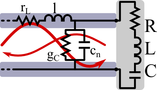
Remember that we found from Kirchhoffs laws the following relations between voltage and current of the transmission line:
\[\begin{eqnarray*} \partial_{x}U\left(x,\omega\right)&=&-\left(r_{L}-\mathrm{i}\omega l\right)I\left(x,\omega\right)\ ,\\\partial_{x}I\left(x,\omega\right)&=&-\left(g_{C}-\mathrm{i}\omega c\right)U\left(x,\omega\right)\ . \end{eqnarray*}\]
With the help of the hint on Kirchoffs law, let us understand impedance matching!
Characteristic Impedance of the Transmission Line
The solutions of the one dimensional Helmholtz equation \(\left(\partial_{xx}+k^{2}\left(\omega\right)\right)U\left(x,\omega\right)=0\) are given by travelling waves:
\[\begin{eqnarray*} U\left(x,\omega\right)&=&U_{0}^{+}\left(\omega\right)e^{\mathrm{i}k\left(\omega\right)x}+U_{0}^{-}\left(\omega\right)e^{-\mathrm{i}k\left(\omega\right)x}\ ,\\U\left(0,\omega\right)&=&U_{0}^{+}\left(\omega\right)+U_{0}^{-}\left(\omega\right)\ . \end{eqnarray*}\]
We use the complex (phasor) notation here. The definition of the sign in the Fourier transformation then defines what in- and outwards propagating solutions are. We shall use a convention in which in time space a wave propagating in positive \(x\) direction is given by some dependency \(\propto\exp\left[\mathrm{i}\left(kx{\color{red}-}\omega t\right)\right]\).
Unfortunately, sometimes other sign conventions are use as in most books on electrical engineering. Luckily, though, a change always only affects the sign of the imaginary unit \(\mathrm{i}\). As a rule of thumb, we just have to replace \(\mathrm{i}\rightarrow-\mathrm{j}\) to convert between the conventions.
Coming back to our actual problem, we have to find the characteristic impedance relating voltage and current of one mode. Since we already know how the voltage looks like, we find the current by the relation
\[\begin{eqnarray*} I\left(x,\omega\right)&=&\frac{1}{\mathrm{i}\omega l-r_{L}}\partial_{x}U\left(x,\omega\right)\ ,\\&=&\frac{1}{\mathrm{i}\omega l-r_{L}}\left[\mathrm{i}k\left(\omega\right)U_{0}^{+}\left(\omega\right)e^{\mathrm{i}k\left(\omega\right)x}-\mathrm{i}k\left(\omega\right)U_{0}^{-}\left(\omega\right)e^{-\mathrm{i}k\left(\omega\right)x}\right]\end{eqnarray*}\]
which we already knew from our considerations of the transmission line following Kirchhoffs laws. Now the current also follows the Helmholtz equation and must have the same wave solutions as the voltage,
\[\begin{eqnarray*} I\left(x,\omega\right)&=&I_{0}^{+}\left(\omega\right)e^{\mathrm{i}k\left(\omega\right)x}+I_{0}^{-}\left(\omega\right)e^{-\mathrm{i}k\left(\omega\right)x} \ . \end{eqnarray*}\]
So, taking \(x=0\), we find
\[\begin{eqnarray*} Z_{0}\left(\omega\right)&=&\frac{V_{0}^{+}\left(\omega\right)}{I_{0}^{-}\left(\omega\right)}=\frac{\mathrm{i}\omega l-r_{L}}{\mathrm{i}k\left(\omega\right)}\\&=&\frac{\mathrm{i}\omega l-r_{L}}{\mathrm{i}\sqrt{-\left(r_{L}-\mathrm{i}\omega l\right)\left(g_{C}-\mathrm{i}\omega c\left(x\right)\right)}}\ . \end{eqnarray*}\]
Here we have employed \(k\left(\omega\right)\). Using the legendary \(\mathrm{i}=\sqrt{-1}\) and cancelling the per unit length, we arrive at the characteristic impedance of a transmission line:
\[\begin{eqnarray*} Z_{0}\left(\omega\right)&=&\sqrt{\frac{\mathrm{i} \omega L^{\prime}-R_{L}}{\mathrm{i}\omega C^{\prime}-G_{C}}} \end{eqnarray*}\]
inserting some primes to not get confused with the oscillating circuit. Note that in general \(L^{\prime}\) and \(C^{\prime}\) will also depend on the frequency.
Voltage Reflection Coefficient and Impedance Matching
To find the voltage reflection coefficient we have to figure out the ratio of reflected voltage amplitude \(U_{0}^{-}\left(\omega\right)\) to the transmitted one \(U_{0}^{+}\left(\omega\right)\) assuming a certain load with impedance (full!) \(Z_{L}\left(\omega\right)=U_{L}\left(\omega\right)/I_{L}\left(\omega\right)\).
First of all, we can use the characteristic impedance of the transmission line to express voltage and current:
\[\begin{eqnarray*} U\left(x,\omega\right)&=&U_{0}^{+}\left(\omega\right)e^{\mathrm{i}k\left(\omega\right)x}+U_{0}^{-}\left(\omega\right)e^{-\mathrm{i}k\left(\omega\right)x}\ ,\\I\left(x,\omega\right)&=&\frac{U_{0}^{+}\left(\omega\right)}{Z_{0}\left(\omega\right)}e^{\mathrm{i}k\left(\omega\right)x}-\frac{U_{0}^{-}\left(\omega\right)}{Z_{0}\left(\omega\right)}e^{-\mathrm{i}k\left(\omega\right)x}\ . \end{eqnarray*}\]
Then we know that at \(x=0\), both voltage and current are continuous:
\[\begin{eqnarray*} U_{0}^{+}\left(\omega\right)+U_{0}^{-}\left(\omega\right)&=&U_{L}\left(\omega\right)\ ,\\\frac{U_{0}^{+}\left(\omega\right)}{Z_{0}\left(\omega\right)}-\frac{U_{0}^{-}\left(\omega\right)}{Z_{0}\left(\omega\right)}&=&I_{L}\left(\omega\right)\ . \end{eqnarray*}\]
This allows us to incorporate the impedance of the load as
\[\begin{eqnarray*} Z_{L}\left(\omega\right)=\frac{U_{L}\left(\omega\right)}{I_{L}\left(\omega\right)}&=&\frac{U_{0}^{+}\left(\omega\right)+U_{0}^{-}\left(\omega\right)}{U_{0}^{+}\left(\omega\right)-U_{0}^{-}\left(\omega\right)}Z_{0}\left(\omega\right)\\&=&\frac{1+\Gamma\left(\omega\right)}{1-\Gamma\left(\omega\right)}Z_{0}\left(\omega\right)\ . \end{eqnarray*}\]
Were we have inserted the voltage reflection coefficient \(\Gamma\left(\omega\right)=U_{0}^{-}\left(\omega\right)/U_{0}^{+}\left(\omega\right)\). The latter equation can finally be solved for the reflection coefficient yielding
\[\begin{eqnarray*} \Gamma\left(\omega\right)&=&\frac{Z_{L}\left(\omega\right)-Z_{0}\left(\omega\right)}{Z_{L}\left(\omega\right)+Z_{0}\left(\omega\right)}\ . \end{eqnarray*}\]
Now we can come to the impedance matching. All the energy is supplied to the load if the reflection coefficient vanishes, thus \(Z_{L}\left(\omega\right)=Z_{0}\left(\omega\right)\). So, for a lossless transmission line and a serial oscillator circuit as load we find the condition
\[\begin{eqnarray*} \sqrt{\frac{L^{\prime}}{C^{\prime}}}&=&R+\frac{\mathrm{i}}{\omega C}-\mathrm{i}\omega L\ . \end{eqnarray*}\]
This conditions must hold both for the imaginary and real part, so:
\[\begin{eqnarray*} LC=\frac{1}{\omega^{2}}&\ \mathrm{and}\ &R=\sqrt{\frac{L^{\prime}}{C^{\prime}}}\ . \end{eqnarray*}\]
Hence we find that we can transfer all of the energy to the circuit only if it is driven at resonance and the resistance corresponds to the (real) impedance of the transmission line.
Already this little example shows how much experience and effort in the development of electrical devices lies. One can imagine that things get much more complicated for realistic scenarios with losses in the transmission line and a lot of constraints from some production and design processes.