Tags: Telegrapher's equation / Kirchhoff's law
![]() We consider a transmission line in a lumped model. This will allow you to find the so-called telegrapher equation which describes the signal propagation along transmission lines in general. You will also see how such devices can even also be used as quantum bits.
We consider a transmission line in a lumped model. This will allow you to find the so-called telegrapher equation which describes the signal propagation along transmission lines in general. You will also see how such devices can even also be used as quantum bits.
Problem Statement
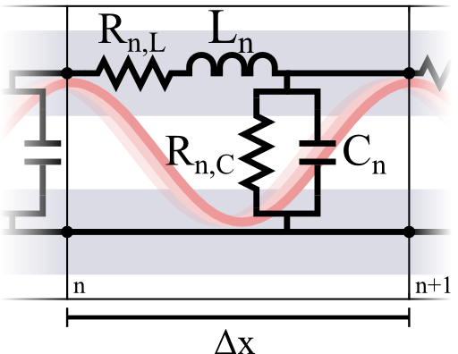
We may regard a transmission line as made up of certain serially connected elements. Each of these elements has length Δx and obeys some lossy inductance Ln (with resistance Rn,L and capacitance Cn (with conductance Gn,C = 1/Rn,C), see figure:
1. Show that in a continuum limit Δx → 0 both voltage and current follow a so-called telegrapher equation
\[\text{(1)}\ \ \partial_{xx}U\left(x,t\right)- a_1 U\left(x,t\right)- a_2\dot{U}\left(x,t\right)- \frac{1}{v^{2}}\ddot{U}\left(x,t\right) = 0\ .\]
(a) Start with Kirchhoffs voltage and current laws to derive a finite-difference equation in space.
(b) Perform the continuum-limit to include spatial derivatives. You should arrive at coupled first-order partial differential equations for voltage and current. You may want to use the characteristic values per length like rC = RC/Δx etc.
(c) Use a representation in “frequency space” (Fourier transform for t → ω to decouple the equations. Assume that the characteristic values are constants. Go back to a time representation to find equation (1) and identify the ai and v.
2. The lossless rL = gC = 0 telegrapher equation is equal to the wave equation
\[\partial_{xx}U \left(x,t\right)-\frac{1}{v^{2}}\ddot{U}\left(x,t\right) = 0\ .\]
For which α is \(U\left(x,t\right)= f\left(x\pm\alpha t\right)\) a solution to this equation?
Discuss your result - what is the implication for signals broadcasted along the transmission line?
Hints
You may want to use that a Fourier transform connecting time- and frequency representation defined as
\[\begin{eqnarray*} f\left(\omega\right)& = &\mathcal{F}\left[f\left(t\right)\right]\left(\omega\right) = \frac{1}{2\pi}\int_{-\infty}^{\infty}e^{\mathrm{i}\omega t}f\left(t\right)dt \end{eqnarray*}\]
converts a time-derivative in a linear partial differential equation into a multiplication with -iω.
You can show this relation using an integration by parts.
Solution ✔
First of all, Kirchhoffs laws and the continuum limit \(\Delta x\rightarrow0\) will give us coupled partial differential equations in voltage and current. We will uncouple these equations in the frequency domain. Switching back to the time domain we will arrive at the telegrapher equation. Finally, we may discuss some implications of this equation for practical signal broadcastings.
Kirchhoffs Laws and Continuum Limit
Kirchhoffs laws for voltage and currents tells us the voltage and current drops from element \(n\) to \(n+1\) to be
\[\begin{eqnarray*}U_{n+1}\left(t\right)&= &U_{n}\left(t\right)-R_{n,L}I_{n}\left(t\right)-L_{n}\dot{I}_{n} \left(t\right)\ ,\mathrm{and}\\ I_{n+1} \left(t\right)& = &I_{n}\left(t\right)-G_{n,C}U_{n}\left(t\right)- C_{n}\dot{U}_{n} \left(t\right)\ . \end{eqnarray*}\]
Now, performing the limit of very small cells of length \(\Delta x\) we find first derivatives in \(x\):
\[\begin{eqnarray*} \lim_{\Delta x\rightarrow0} \frac{U_{n+1}\left(t\right)- U_{n}\left(t\right)}{\Delta x}\equiv \partial_{x}U\left(x,t\right)&=&-r_{L}\left(x\right)I \left(x,t\right)-l\left(x\right)\dot{I}\left(x,t \right)\ ,\\\partial_{x}I\left(x,t\right)&=&-g_{C} \left(x\right)U \left(x,t\right)-c\left(x\right)\dot{U} \left(x,t\right) \end{eqnarray*}\]
using the characteristics like resistance in units per length.
Frequency Space
A Fourier transformation, which we shall define as
\[f\left(\omega\right) = \mathcal{F}\left[f\left(t\right)\right]\left(\omega\right)=\frac{1}{2\pi}\int_{-\infty}^{\infty}e^{\mathrm{i}\omega t}f\left(t\right)dt\ ,\]
converts the time derivative \(\partial_{t}\) into \(-\mathrm{i}\omega\). We may see this from a quick integration by parts assuming that \(f\left(t\right)\rightarrow0\) for \(\omega\rightarrow\pm\infty\):
\[\begin{eqnarray*} \mathcal{F}\left[\partial_{t}f \left(t\right)\right]\left(\omega\right)& = &\frac{1}{2\pi} \int_{-\infty}^{\infty}e^{\mathrm{i}\omega t}\left(\partial_{t}f\left(t\right) \right)dt\\& = &-\frac{1}{2\pi} \int_{-\infty}^{\infty} \left(\partial_{t}e^{\mathrm{i}\omega t} \right)f\left(t\right)dt+\frac{1}{2\pi}\left.e^{\mathrm{i} \omega t} f\left(t\right)\right|_{-\infty}^{\infty}\\& = &-\mathrm{i} \omega\frac{1}{2\pi} \int_{-\infty}^{\infty}\left(\partial_{t}e^{\mathrm{i}\omega t}\right)f\left(t\right)dt\\& = &-\mathrm{i}\omega \mathcal{F} \left[f\left(t\right)\right] \left(\omega\right)\ . \end{eqnarray*}\]
So we find in frequency space
\[\begin{eqnarray*} \partial_{x}U\left(x,\omega\right)& = &-\left(r_{L}\left(x\right)-\mathrm{i}\omega l\left(x\right)\right)I\left(x,\omega\right)\ ,\\\partial_{x}I\left(x,\omega\right)&=&-\left(g_{C}\left(x\right)-\mathrm{i}\omega c\left(x\right)\right)U\left(x,\omega\right)\ . \end{eqnarray*}\]
We can directly read-off the solution as
\[\begin{eqnarray*} \partial_{xx}U\left(x,\omega\right)&=&\left(r_{L}\left(x\right)- \mathrm{i}\omega l\left(x\right)\right)\left(g_{C}\left(x\right)-\mathrm{i}\omega c\left(x\right)\right)U\left(x,\omega\right) \end{eqnarray*}\]
where the same equation holds for the current.
The Telegraphers Equation
Now, coming back into the time-domain we find, replacing \(\mathrm{-}\mathrm{i}\omega\rightarrow\partial_{t}\)
\[\begin{eqnarray*} \partial_{xx}U\left(x,t\right)& = &\left(r_{L}\left(x\right)+l\left(x\right)\partial_{t}\right)\left(g_{C}\left(x\right)+c\left(x\right)\partial_{t}\right)U\left(x,t\right)\ . \end{eqnarray*}\]
Now, factoring out, we find:
\[\begin{eqnarray*}\text{(2)}\ \ \partial_{xx}U\left(x,t\right)-r_{L}\left(x\right)g_{C} \left(x\right)U\left(x,t\right)- \left(r_{L}\left(x\right)c\left(x\right)+g_{C} \left(x\right)l\left(x\right)\right) \dot{U}\left(x,t\right)- \frac{1}{v^{2}\left(x\right)}\ddot{U}\left(x,t\right)& = &0\end{eqnarray*}\]
with space-dependent
\[\begin{eqnarray*} v^{2}\left(x\right)&=&\frac{1}{l\left(x\right)c\left(x\right)}=\frac{\Delta x^{2}}{L_{n\left(x\right)}C_{n\left(x\right)}}=\omega_{0}^{2}\left(x\right)\Delta x^{2}\ . \end{eqnarray*}\]
We will see soon what kind of interpretation \(v\) has.
We can already see that the pre-factors in equation (2) are position dependent. So we may have derived something rather general. However, if these are all constants, the equation we found is indeed the telegraph(er's) equation (or damped-wave equation),
\[\begin{eqnarray*} \partial_{xx}U\left(x,t\right)- r_{L}g_{C}U\left(x,t\right)-\left(r_{L}c +g_{C}l\right)\dot{U}\left(x,t\right)-\frac{1}{v^{2}}\ddot{U}\left(x,t\right)&=&0\ . \end{eqnarray*}\]
Here, we may also directly read-off the constants \(a_i\).
Wave Propagation
At last we want to consider the telegrapher equation without losses, \(r_{L}=g_{C}=0\):
\[\begin{eqnarray*} \partial_{xx}U\left(x,t\right)- \frac{1}{v^{2}}\ddot{U}\left(x,t\right)&=&0\ .\end{eqnarray*}\]
If we insert the trial function \(f\left(x\pm\alpha t\right)\), we find that
\[\begin{eqnarray*} f^{\prime\prime}\left(x\pm\alpha t\right)- \frac{\alpha^{2}}{v^{2}}f^{ \prime\prime}\left(x\pm\alpha t\right)&= &0\ \mathrm{,\ so}\\ \alpha&\equiv&v\ . \end{eqnarray*}\]
Since \(f\left(x\pm\alpha t\right)\) describes some function propagating in negative (positive) \(x\)-direction in time at some velocity \(\alpha\), we can likewise interpret \(v=1/\sqrt{lc}\) as the velocity at which signals of any arbitrary form are transmitted along the transmission line. (Remember: the capacitance per length is called \(c\) here and shall not be confused with the speed of light.)

This is, however, only half of the story. In reality, we might split a signal into its frequency components by the Fourier transform. The transmission line will have a velocity depending on the frequency of every component. Then we should better write the lossless telegrapher equation in this domain,
\[\begin{eqnarray*} \partial_{xx}U\left(x,\omega\right)+ l\left(\omega\right)r\left( \omega\right)\omega^{2}U\left(x,\omega\right)& = &0\ . \end{eqnarray*}\]
The result will be that signals will get distorted in some way which is called dispersion. We will re-encounter this effect later on in problems related to wave propagation in media - there is a lot more to say about it.
Background: Superconducting Transmission Lines for Quantum Computation
 Let us think about some applications of transmission lines. There are the obvious ones in the radio-frequency domain but we may go a little bit deeper here to fundamental physics. We will see that superconducting transmission lines might be used as quantum bits in quantum computers.
First, a very handwaving summary of the Bardeen, Cooper and Schrieffer (BCS) theory of superconductivity. The interactions of phonons to electrons results in an effective attraction between electrons. Such coupled electrons are called a Cooper pair and are Bosons, not Fermions like a single electron. Bosons have quantum-mechanically different properties (no Pauli-principle!) and can propagate through a solid state body without resistance. (More on a description of superconductivity in terms of massive photons can be found in the background of Superconductors and Their Magnetostatic Fields.)
If one puts two superconductors close together, they form a cavity in-between. Through this cavity, Cooper-pairs can tunnel to the other side which is called Josephson effect. This effect enables a certain coupling between the two superconducting sides. In a classical picture, if two electrons were tunneling, there will be an electric field between them. Assuming that the tunneling is not very frequent such that only none or one pair is crossed at any time, the superconductors with Cooper pairs are basically a two-level system.
On the contrary, if an electric field is present between the two superconductors, this field may couple to the Cooper pairs. The interaction to the transmission line then allows for example to switch between the states of this two-level-system. This makes the superconductors an accessible quantum bit, the analog to a classical bit! This setup is indeed a promising candidate as a building block for quantum computers. Much more details can be found in “Cavity quantum electrodynamics for superconducting electrical circuits: an architecture for quantum computation” by Blais et al., Physical Review A 69 (2004).
Journal Page | arXiv | PDF
</div>