An Electric Charge in front of a Dielectric Interface

The method of image charges can also be applied to problems including dielectrics. In this problem, a charge in front of an interface between two dielectrics is considered. Find out how to solve it and what happens if the charge is put in between the dielectrics.

Problem Statement

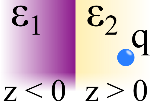
Let us assume two dielectric media with permittivities ε₁ for z < 0 and ε₂ for z > 0.

In r_q = (x_q,y_q,d) may be a charge q.

Calculate the electrostatic potential ϕ(r) for the whole space.

Furthermore, calculate the electrostatic potential ϕ(r) in the limit d → 0 and discuss your result.

On the right is a schematic of the situation:

Hints

Can you explain the physical effect of the charge in this setup?

What are the boundary conditions in electrostatics?

Hopefully the hints were somewhat useful! Let us calculate the electrostatic potential for this "two-world" scenaria!

Solution

To solve the given problem and determine the potential, we may first find a suitable ansatz for ϕ(r) employing the method of image charges.

After we have done this primary step we will be able to use the boundary conditions to determine the so-far unknown image charges.

At last we can have a look what happens if we are able to place the charge directly on the boundary.

The Potential in terms of Image Charges

As usuall we assume a linear relationship between electric field and electric displacement field. Note that strictly speaking this relationship should be clarified in the problem statement. However, if permittivities are given, one can always assume that this refers to the linear relationship

\[\begin{eqnarray*}\mathbf{D} & = & \varepsilon \mathbf{E}\ .\end{eqnarray*}\]

So let us calculate the electrostatic potential employing the method of image charges. As always is very helpful to first picture what is happening physically. Because of the point charge, in both media will be an induced polarization field. Furthermore, there will be a surface charge density at the boundary. We now have to represent this surface charge density by image charges of unknown values. Remember that these image charges are not real. So we have to construct the solution as a combination of solutions for those regions where we did not use image charges, i.e.\[\begin{eqnarray*}\phi \left(\mathbf{r}\right) & = & \begin{cases}\phi_2 \left(\mathbf{r}\right) \ , & z>0\\ \phi_1 \left(\mathbf{r}\right)\ , & z<0\end{cases}\end{eqnarray*}\]The respective values of the image charges will be determined by the boundary conditions.

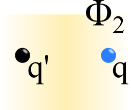First we want to find a solution for \(z>0\). We may represent the surface charge density by the image charge \( q^\prime\) at \(\mathbf{r}_{q^\prime} = \left(x_q,y_q,-d\right)\) to find \(\phi_2\), see right figure.

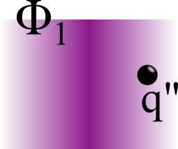
We make the same approach for the potential \(\phi_1\) with some image charge at the original charge position (left figure). You might ask why we cannot just take the original charge here. The point ist that the induced surface charge "screens" the original charge. We have to fully account for this effect.

Let us write down the potential in our approach with the still unknown charges: \[\begin{eqnarray*}\phi\left(\mathbf{r}\right) & = & \begin{cases}\phi_{2}=\frac{1}{4\pi\varepsilon_{2}}\left(\frac{q}{R_{-}}+\frac{q'}{R_{+}}\right)\ , & z>0\\ \phi_{1}=\frac{1}{\ 4\pi\varepsilon_{1}}\cdot\frac{q''}{R_{-}}\ , & z<0\end{cases}\ \mathrm{with}\\R_{\pm} & = & \sqrt{x^{2}+y^{2}+\left(z\pm d\right)^{2}}\ .\end{eqnarray*}\]So, all we have to do is to calculate the two image charges from the boundary conditions.

Solving the Boundary Conditions to Determine Image Charges

The boundary conditions at \(z=0\) are now given by\[\begin{eqnarray*}\varepsilon_{1}E_{z}^{1} & = & \varepsilon_{2}E_{z}^{2}\\E_{x}^{1} & = & E_{x}^{2}\\E_{y}^{1} & = & E_{y}^{2}\end{eqnarray*}\] or in \(\phi\) using \[\begin{eqnarray*}\mathbf{E} & = & -\mathrm{grad}\phi\ .\end{eqnarray*}\]Since now \[\begin{eqnarray*}\frac{\partial}{\partial z}\frac{1}{R_{\pm}} & = & -\frac{z\pm d}{R_{\pm}^{3}}\ ,\\ \left.\frac{\partial}{\partial z}\frac{1}{R_{\pm}}\right|_{z=0} & = & \mp\frac{d}{R_{\pm}^{3}\left(x,y,z=0\right)}\ \mathrm{and}\\ R_{+}\left(x,y,0\right) & = & R_{-}\left(x,y,0\right)\ ,\end{eqnarray*}\]we find for the first boundary condition \[\begin{eqnarray*}4\pi\varepsilon_{2}E_{z}^{2} & = & 4\pi\varepsilon_{2}\partial_{z}\phi_{2}\\ & = & \partial_{z}\left(\frac{q}{R_{-}}+\frac{q'}{R_{+}}\right)\ ,\\ 4\pi\varepsilon_{1}E_{z}^{1} & = & 4\pi\varepsilon_{1}\partial_{z}\phi_{1}\\ & = & \partial_{z}\left(\frac{q''}{R_{-}}\right)\ ,\ \mathrm{also}\\ q-q' & = & q''\ .\end{eqnarray*}\]

The derivation with respect to \(x\) and \(y\) do not result in any sign change. So, because of the continuity of \(\partial_{\left(x,y\right)}\phi\) we find \[\begin{eqnarray*}\frac{1}{\varepsilon_{2}}\left(q+q'\right) & = & \frac{q''}{\varepsilon_{1}}\ \mathrm{so}\\ q' & = & -\frac{\varepsilon_{1}-\varepsilon_{2}}{\varepsilon_{1}+\varepsilon_{2}}\cdot q\ ,\\ q'' & = & \frac{2\varepsilon_{1}}{\varepsilon_{1}+\varepsilon_{2}}\cdot q\ . \end{eqnarray*}\]Now we have determined all unknown image charges - we have calculated the field entirely. But what happens if the charge is placed directly between both dielectrics?

The Charge in-between the Dielectrics

Now to the last part of the problem. \(d\rightarrow0\) leads to \(R_{\pm}\rightarrow r=\sqrt{x^{2}+y^{2}+z^{2}}\) and hence\[\begin{eqnarray*}\phi & \rightarrow & \begin{cases}\phi_{2}=\frac{1}{4\pi\varepsilon_{2}}\cdot\frac{q+q'}{r}\ , & z>0\\ \phi_{1}=\frac{1}{\ 4\pi\varepsilon_{1}}\cdot\frac{q''}{r}\ , & z<0\end{cases}\\ & = & \frac{1}{4\pi\varepsilon_{0}\tilde{\varepsilon}_{r}}\cdot\frac{q}{r}\ \forall \mathbf{r}\ \mathrm{with}\\ \tilde{\varepsilon}_r & = & \frac{1}{2}\left(\varepsilon_{1}+\varepsilon_{2}\right)\ .\end{eqnarray*}\]This result is astonishing. The limiting process leads to an effective medium with permittivity \(\tilde{\varepsilon}_r\) or a vacuum with charge \(q/\tilde{\varepsilon}_{r}\).