Tags: Rotational Symmetry / Quadrupole Moment / Legendre Polynomials
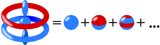
![]() In rotational symmetry, the multipole moments of a charge distribution are described by just one component per order l. This is a drastic difference to the usual 2l + 1 independent components. Get to know this simplifications with two examples and derive it for any charge distribution with rotational symmetry!
In rotational symmetry, the multipole moments of a charge distribution are described by just one component per order l. This is a drastic difference to the usual 2l + 1 independent components. Get to know this simplifications with two examples and derive it for any charge distribution with rotational symmetry!
Problem Statement
A charge distribution shall obey rotational symmetry with respect to the z axis, see schematic below:
Proof that its multipole moments are entirely given by its components with respect to the axis of symmetry.
So, the dipole moment just depends on its z component ρz, the quadrupole moment on Qzz. and so on. Let us approach this very useful conclusion in two steps:
1. Examples:
a) Show that the dipole moment is given by p = pzez.
b) Calculate that the cartesian quadrupole tensor is diagonal and that
\[Q_{xx}=Q_{yy}=-\frac{1}{2}Q_{zz}\text{ holds.}\]
2. Proof of the general conclusion:
a) Derive that the general solution of the electrostatic potential outside of the charge distribution is given by
\[\phi\left(r,\theta\right) = \frac{1}{4\pi\varepsilon_{0}}\sum_{l=0}^{\infty}\frac{b_{l}P_{l}\left(\cos\theta\right)}{r^{l+1}}\]
using a separation of variables in spherical coordinates. Note that the so-called Legendre Polynomials \(P_{l}\left(\cos\theta\right)\) are given by the differential equation
\[\frac{1}{\sin\theta}\frac{d}{d\theta}\sin\theta\frac{d}{d\theta}P_{l}\left(\cos\theta\right)+l\left(l+1\right)P_{l}\left(\cos\theta\right) = 0\ ,\]
where only a solution exists if \(l\in\mathbb{N}_{0}=\left\{ 0,\ 1,\ 2,\ \dots\right\}\).
b) Use \(P_{l}\left(\cos\theta=1\right)=1\ \forall l\) and
\[\frac{1}{\sqrt{1-2\xi\cos\theta+\xi^{2}}} \equiv \sum_{l=0}^{\infty}P_{l}\left(\cos\theta\right)\xi^{l}\]
to show that the multipole moments are given by
\[b_{l} = \int P_{l}\left(\cos\theta^{\prime}\right)r^{\prime l}\rho\left(r^{\prime},\theta^{\prime}\right)dV^{\prime}\ .\]
Hints
1. You do not need to show that the quadrupole tensor is traceless, you may use it directly.
2. a) The electrostatic potential obeys the Laplace equation \(\Delta\phi\left(\mathbf{r}\right) = 0\) outside of the charge distribution.
What does the given symmetry of the charge distribution imply for the potential? The Laplace operator is separable in spherical coordinates which means that
\[\Delta\phi\left(\mathbf{r}\right)\text{ can be solved by }\phi\left(\mathbf{r}\right)=f\left(r\right)P\left(\theta\right)\psi\left(\varphi\right)\ .\]
A power series expansion is a powerful tool to solve certain differential equations.
2. b) Remember that the electrostatic potential is generally given by
\[\phi\left(\mathbf{r}\right) = \frac{1}{4\pi\varepsilon_{0}}\int\frac{\rho\left(\mathbf{r}^{\prime}\right)}{\left|\mathbf{r}-\mathbf{r}^{\prime}\right|}dV^{\prime}\ .\]
Solution
Let's first see if the multipole moments are determined by only one component first for the dipole and quadrupole and afterwards totally general.
1. Examples - Dipole and Quadrupole in Rotational Symmetry
a) Dipole Moment
Let us consider the dipole moment first since it can be done fast.
Let us perform the actual integration in cylindrical coordinates (r, θ, φ).
In this coordinate syste, the volume element is given by dV = r dφ dr dz. Then, we determine the cartesian dipole moment as
\[\begin{eqnarray*} \mathbf{p}&=&\int\mathbf{r}\rho\left(\mathbf{r}\right)dV\\&=&\int_{-\infty}^{\infty}\int_{0}^{\infty}\int_{0}^{2\pi}\left(\begin{array}{c}r\cos\varphi\\r\sin\varphi\\z\end{array}\right)\rho\left(r,z\right)rd\varphi drdz\\&=&p_{z}\mathbf{e}_{z}\ , \end{eqnarray*}\]
since the integrations over the sine and cosine will just vanish. So, ok, we only have the z-component for the dipole in rotational symmetry. What about the quadrupole, does the knowledge of Qzz suffice to know the whole tensor?
b) Quadrupole Moment
The symmetric and traceless (!) quadrupole tensor is generally defined as
\[\begin{eqnarray*} Q_{ab}&=&\int\left(3x_{a}x_{b}-r^{2}\delta_{ij}\right)\rho\left(\mathbf{r}\right)dV\ \text{with}\\x_{a,b,c}&=&x,\ y\ \text{or }z\ . \end{eqnarray*}\]
Let us first look if the off-diagonal terms vanish if the charge distribution is rotationally symmetric around the z axis:
\[\begin{eqnarray*} Q_{xy}&=&\int3xy\rho\left(\mathbf{r}\right)dV\\&=&3\int_{-\infty}^{\infty}\int_{0}^{\infty}\underbrace{\int_{0}^{2\pi}\cos\varphi\sin\varphi d\varphi}_{=0}\rho\left(r,z\right)r^{3}drdz=0\ . \end{eqnarray*}\]
The same holds for the other off-diagonal terms:
\[\begin{eqnarray*} Q_{xz}&=&3\int_{-\infty}^{\infty}\int_{0}^{\infty}\underbrace{\int_{0}^{2\pi}\cos\varphi d\varphi}_{=0}\rho \left(r,z\right)zr^{2}drdz=0\ \text{and}\\Q_{yz}&=&3\int_{-\infty}^{\infty}\int_{0}^{\infty}\underbrace{\int_{0}^{2\pi}\sin\varphi d\varphi}_{=0}\rho\left(r,z\right)zr^{2}drdz=0\ . \end{eqnarray*}\]
Now to the diagonal components:
\[\begin{eqnarray*} Q_{xx}&=&\int\left(3x^{2}-r^{2}\right)\rho\left(\mathbf{r}\right)dV\\&=&\int_{-\infty}^{\infty}\int_{0}^{\infty}\int_{0}^{2\pi}\left(3\cos^{2}\varphi-1\right)d\varphi\rho\left(r,z\right)r^{3}drdz\ . \end{eqnarray*}\]
The actual value of the \(\varphi\)-integration,
\[\int_{0}^{2\pi}\left(3\cos^{2}\varphi-1\right)d\varphi = 3\pi-2\pi=\pi\]
is of minor interest here. The only thing that counts is that we find the same value for Qyy since the integral over the squared sine or cosine over the whole circle remains the same:
\[\begin{eqnarray*} Q_{yy}&=&\int\left(3y^{2}-r^{2}\right)\rho\left(\mathbf{r}\right)dV\\&=&\int_{-\infty}^{\infty}\int_{0}^{\infty}\int_{0}^{2\pi}\left(3\sin^{2}\varphi-1\right)d\varphi\rho\left(r,z\right)r^{3}drdz\\&=&Q_{xx}\ . \end{eqnarray*}\]
Do we have to calculate Qzz now explicitly? No - since the quadrupole tensor is traceless, we know that with Qxx = Qyy
\[\begin{eqnarray*} Q_{xx}+Q_{yy}+Q_{zz}&=&0\ \text{becomes}\\Q_{xx}=Q_{yy}&=&-\frac{1}{2}Q_{zz} \end{eqnarray*}\]
as desired. But this cannot be a coincidence! Again we have that in rotational symmetry the entire moment is just determined by its component with respect to the axis of symmetry! We have to investigate this fact to find that this is a very general behaviour!
2. Proof of the General Conclusion
a ) Rotationally Symmetric Charge Distributions and their Electrostatic Potential
In spherical coordinates,
\[\Delta\phi\left(r,\theta\right) = \left(\frac{1}{r^{2}}\partial_{r}r^{2}\partial_{r}+\frac{1}{r^{2}\sin\theta}\partial_{\theta}\sin\theta\partial_{\theta}+\frac{1}{r^{2}\sin^{2}\theta}\partial_{\varphi\varphi}\right)\phi\left(r,\theta\right)\]
now the last derivative with respect to φ vanishes. Outside of the charge configuration, the potential satisfies the Laplace equation. We may try to solve it by separation of variables:
\[\begin{eqnarray*} \phi\left(r,\theta\right)&=&f\left(r\right)P\left(\theta\right)\ ,\ \text{so}\\\Delta\phi\left(r,\theta\right)&=&\frac{P\left(\theta\right)}{r^{2}}\partial_{r}r^{2}\partial_{r}f\left(r\right)+\frac{f\left(r\right)}{r^{2}\sin\theta}\partial_{\theta}\sin\theta\partial_{\theta}P\left(\theta\right)=0\ ,\\\frac{1}{f\left(r\right)}\partial_{r}r^{2}\partial_{r}f\left(r\right)&=&-\frac{1}{P\left(\theta\right)\sin\theta}\partial_{\theta}\sin\theta\partial_{\theta}P\left(\theta\right)\equiv\alpha\ . \end{eqnarray*}\]
Both sides have to be constant since either side is depending on different (indepent) variables - r and θ, respectively.
Note that the Laplace equation, a partial differential equation becomes two homogeneous differential equations, a quite remarkable simplification - we may use standard methods to solve them (... or look up their solutions :).
Now we know from the problem that the Legendre differential equation,
\[\frac{1}{\sin\theta}\frac{d}{d\theta}\sin\theta\frac{d}{d\theta}P_{l}\left(\cos\theta\right)+\alpha P_{l}\left(\cos\theta\right) = 0\ ,\]
can only have solutions for \(\theta=\left\{ 0,\pi\right\}\), if \(\alpha = l\left(l+1\right)\ \text{with }l\in\mathbb{N}_{0}\).
Here, the natural integers \(\mathbb{N}_{0}=\left\{ 0,\ 1,\ 2,\ \dots\right\}\) are used.
The solutions are called Legendre Polynomials and the first three are given by:
\[\begin{eqnarray*} P_{0}\left(\cos\theta\right)&=&1\\P_{1}\left(\cos\theta\right)&=&\cos\theta\\P_{2}\left(\cos\theta\right)&=&\frac{1}{2}\left(3\cos^{2}\theta-1\right)\ . \end{eqnarray*}\]
Now we still have to solve the differential equation for f(r):
\[\begin{eqnarray*} \frac{d}{dr}r^{2}\frac{d}{dr}f\left(r\right)&=&l\left(l+1\right)f\left(r\right)\ \text{, so}\\r^{2}f^{\prime\prime}\left(r\right)+2rf^{\prime}\left(r\right)-l\left(l+1\right)f\left(r\right)&=&0\ . \end{eqnarray*}\]
We use a power series expansion and check if we obtain the correct results:
\[\begin{eqnarray*} f\left(r\right)&=&\sum_{l=0}^{\infty}\color{red}{a_{l}}r^{l}+\frac{\color{green}{b_{l}}}{r^{l+1}}\ ,\\\color{red}{a_{l}}:\quad0&=&r^{2}l\left(l-1\right)a_{l}r^{l-2}+2rla_{l}r^{l-1}-l\left(l+1\right)a_{l}r^{l}\\&=&r^{l}a_{l}\left[l\left(l-1\right)+2l-l\left(l+1\right)\right]=0\ \surd\\\color{green}{b_{l}}:\quad0&=&r^{2}\left(l+1\right)\left(l+2\right)\frac{b_{l}}{r^{l+3}}-2r\left(l+1\right)\frac{b_{l}}{r^{l+2}}-l\left(l+1\right)\frac{b_{l}}{r^{l+1}}\\&=&\frac{b_{l}}{r^{l+1}}\left[\left(l+1\right)\left(l+2\right)-2\left(l+1\right)-l\left(l+1\right)\right]=0\ \surd\ . \end{eqnarray*}\]
This is of course the general solution to the problem. We are however only interested in solutions outside of the source and vanishing at infinity. Then we can only keep the bl-terms and obtain the general solution for the electrostatic potential charge distributions with rotational symmetry as
\[\phi\left(r,\theta\right) = \frac{1}{4\pi\varepsilon_{0}}\sum_{l=0}^{\infty}\frac{b_{l}P_{l}\left(\cos\theta\right)}{r^{l+1}}\ .\]
Note that the moments of a given order l are given by just one constant as we wanted to proof!
Furthermore we added the usual \(1/4\pi\varepsilon_{0}\)-prefactor just that the moments have the "correct" well-known units and scaling - for example b0 should be just the total charge. This brings us to the next point:
b) Determination of the Multipole Moments in Rotational Symmetry
We know that generally the multipole moments come from the integral formulation of Gauss's law. Let us compare the two formulas with our result for rotational symmetry:
\[\begin{eqnarray*} \phi\left(r,\theta\right)&=&\frac{1}{4\pi\varepsilon_{0}}\int\frac{\rho\left(r^{\prime},\theta^{\prime}\right)}{\left|\mathbf{r}-\mathbf{r}^{\prime}\right|}dV^{\prime}\\&=&\frac{1}{4\pi\varepsilon_{0}}\sum_{l=0}^{\infty}\frac{b_{l}P_{l}\left(\cos\theta\right)}{r^{l+1}}\ \text{(rot. symm.)}. \end{eqnarray*}\]
We can see that the potential is entirely determined by its behaviour on the axis of symmetry: If we take z > 0, this implies θ = 0 where we can use \(P_{n}\left(\cos0=1\right)=1\):
\[\phi\left(r,\theta=0\right) = \frac{1}{4\pi\varepsilon_{0}}\sum_{l=0}^{\infty}\frac{b_{l}}{z^{l+1}}\ \text{(rot. symm.)}.\]
Furthermore,
\[\begin{eqnarray*} \phi\left(r,\theta=0\right)&=&\frac{1}{4\pi\varepsilon_{0}}\int\frac{\rho\left(r^{\prime},\theta^{\prime}\right)}{\left|z\mathbf{e}_{z}-\mathbf{r}^{\prime}\right|}dV^{\prime}\\&=&\frac{1}{4\pi\varepsilon_{0}}\int\frac{\rho\left(r^{\prime},\theta^{\prime}\right)}{\sqrt{z^{2}-2zr^{\prime}\cos\theta^{\prime}+r^{\prime2}}}dV^{\prime} \end{eqnarray*}\]
Here we have used the law of cosines to express the \(1/\left|z\mathbf{e}_{z}-\mathbf{r}^{\prime}\right|\)-term.
This expression brings us directly to the definition of the Legendre Polynomials:
\[\frac{1}{\sqrt{1-2\xi\cos\theta+\xi^{2}}} = \sum_{l=0}^{\infty}P_{l}\left(\cos\theta\right)\xi^{l}\ .\]
Now we can re-formulate the integral for the potential on the axis of symmetry, since
\[\begin{eqnarray*} \frac{1}{\sqrt{z^{2}-2zr^{\prime}\cos\theta^{\prime}+r^{\prime2}}}&=&\frac{1}{z}\frac{1}{\sqrt{1-2\frac{r^{\prime}}{z}\cos\theta^{\prime}+\left(\frac{r^{\prime}}{z}\right)^{2}}}\\&=&\frac{1}{z}\sum_{l=0}^{\infty}P_{l}\left(\cos\theta^{\prime}\right)\left(\frac{r^{\prime}}{z}\right)^{l} \end{eqnarray*}\]
and obtain
\[\begin{eqnarray*}\phi\left(r,\theta=0\right)&=&\frac{1}{4\pi\varepsilon_{0}}\int\frac{\rho\left(r^{\prime},\theta^{\prime}\right)}{\sqrt{z^{2}-2zr^{\prime}+r^{\prime2}}}dV^{\prime}\\&=&\frac{1}{4\pi\varepsilon_{0}}\sum_{l=0}^{\infty}\frac{1}{z^{l+1}}\int P_{l}\left(\cos\theta^{\prime}\right)r^{\prime l}\rho\left(r^{\prime},\theta^{\prime}\right)dV^{\prime}\ .\end{eqnarray*}\]
Then, we can just read off that the multipole moments for a charge distribution with rotational symmetry are given by
\[b_{l} = \int P_{l}\left(\cos\theta^{\prime}\right)r^{\prime l}\rho\left(r^{\prime},\theta^{\prime}\right)dV^{\prime}\ .\]
For l = 0, we find the total charge, b0 = Q, the next term is b1 = pz, i.e. the dipole moment. b2 = Qzz and so on.
In the end we can conclude that the multipole moments are indeed just given by one single moment per order for rotational symmetry! For general charge distributions, there are 2l + 1 independent components for each order...
Furthermore, the moments can be calculated again using the well-known Legendre polynomials as we have successfully demonstrated!
I hope for you this derivation on electrostatic multipole moments in rotational symmetry has been insightful. It demonstrates the power of special functions in mathematical physics, here the Legendre polynomials. You will use such functions over and over again.


