Tags: Harmonic Oscillator / Coupling / Resistance / Inductance / Capacitance
![]() We all know them: twins. Either they love and support each other or they are fighting to find out who is the best. The reason is that they are almost equal. In this problem we will find out why they behave as they do understanding coupled oscillatory circuits.
We all know them: twins. Either they love and support each other or they are fighting to find out who is the best. The reason is that they are almost equal. In this problem we will find out why they behave as they do understanding coupled oscillatory circuits.
Problem Statement
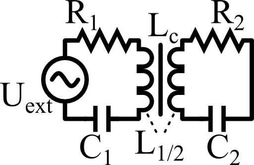 Two RLC-circuits are inductively coupled via an inductance Lc. Determine the currents in both circuits. Under which condition can the currents in both circuits become infinite? Find the corresponding frequencies ω±.
Determine the difference ω+ - ω- if the resonance frequencies of the single circuits are equal.
Calculate this so-called detuning for sufficiently small mutual inductance.
Verify that you find the same results using an eigenfrequency analysis assuming vanishing resistances.
Hints
Start from the coupled differential equations for the circuits. Then switch to frequency space (phasor representation) and solve the algebraic system of equations.
You may need the following Taylor approximations:
\[\sqrt{1-x}\approx1-x/2+\mathcal{O}\left(x^{2}\right)\text{ and}\]
\[1/\sqrt{1-x^{2}}\approx1+x^{2}/2\]
For the eigenfrequency analysis short the voltage supply and find an equation for ω, the characteristic equation.
Let us find the solution to coupled oscillatory circuits!
Determining the Currents
We start, as usual with the integro-differential equations governing the system:
\[\begin{eqnarray*} U_{\mathrm{ext}}\left(t\right)&=&L_{1}\dot{I}_{1}\left(t\right)+R_{1}I_{1}\left(t\right)+\frac{1}{C_{1}}\int_{-\infty}^{t}I_{1}\left(\tau\right)d\tau-L_{c}\dot{I}_{2}\left(t\right)\\0&=&L_{2}\dot{I}_{2}\left(t\right)+R_{2}I_{2}\left(t\right)+\frac{1}{C_{2}}\int_{-\infty}^{t}I_{2}\left(\tau\right)d\tau-L_{c}\dot{I}_{1}\left(t\right)\ . \end{eqnarray*}\]
The most important here is the sign of the coupling term which represents an external voltage source.
To get rid of the integral, we may derive the equations once more with respect to time. Then we have have two linear coupled differential equations.
In this case it is always conventient to go to a Fourier representation to find the algebraic equations
\[\begin{eqnarray*} -\mathrm{i}\omega U_{\mathrm{ext}}\left(\omega\right)&=&\omega^{2}L_{1}I_{1}\left(\omega\right)-\mathrm{i}\omega R_{1}I_{1}\left(\omega\right)+\frac{1}{C_{1}}I_{1}\left(\omega\right)+\omega^{2}L_{c}I_{2}\left(\omega\right)\ \mathrm{and}\\0&=&\omega^{2}L_{2}I_{2}\left(\omega\right)-\mathrm{i}\omega R_{2}I_{2}\left(\omega\right)+\frac{1}{C_{2}}I_{2}\left(\omega\right)+\omega^{2}L_{c}I_{1}\left(\omega\right)\ .\end{eqnarray*}\]
Devision by \(-\mathrm{i}\omega\) results in
\[\begin{eqnarray*} U_{\mathrm{ext}}\left(\omega\right)&=&Z_{1}\left(\omega\right)I_{1}\left(\omega\right)+\mathrm{i}\omega L_{c}I_{2}\left(\omega\right)\\0&=&Z_{2}\left(\omega\right)I_{2}\left(\omega\right)+\mathrm{i}\omega L_{c}I_{1}\left(\omega\right)\ \mathrm{with}\\Z_{i}\left(\omega\right)&=&R_{i}-\mathrm{i}\omega L_{i}+\frac{\mathrm{i}}{\omega C_{i}}\ . \end{eqnarray*}\]
We can read-off
\[\begin{eqnarray*} I_{1}\left(\omega\right)&=&-\frac{Z_{2}\left(\omega\right)}{\mathrm{i}\omega L_{c}}I_{2}\left(\omega\right)\ ,\ \mathrm{so}\\U_{\mathrm{ext}}\left(\omega\right)&=&-\frac{Z_{1}\left(\omega\right)Z_{2}\left(\omega\right)}{\mathrm{i}\omega L_{c}}I_{2}\left(\omega\right)+\mathrm{i}\omega L_{c}I_{2}\left(\omega\right) \end{eqnarray*}\]
and find the solution to the first task of the problem:
\[\begin{eqnarray*} I_{2}\left(\omega\right)&=&\frac{\mathrm{i}\omega L_{c}}{\left[\left(\mathrm{i}\omega L_{c}\right)^{2}-Z_{1}\left(\omega\right)Z_{2}\left(\omega\right)\right]}U_{\mathrm{ext}}\left(\omega\right)\ ,\\I_{1}\left(\omega\right)&=&-\frac{Z_{2}\left(\omega\right)}{\mathrm{i}\omega L_{c}}I_{2}\left(\omega\right)\\&=&-\frac{Z_{2}\left(\omega\right)}{\left[\left(\mathrm{i}\omega L_{c}\right)^{2}-Z_{1}\left(\omega\right)Z_{2}\left(\omega\right)\right]}U_{\mathrm{ext}}\left(\omega\right)\ . \end{eqnarray*}\]
Ok, that was quite some math! we started with the integro-differential equations that govern the system. Then we got rid of the integral by one further derivation. Afterwards we transformed to frequency / Fourier space. Then we were able to find the frequency-dependent currents dependent on the excitation.
If you are a bit overwhelmed right now - don't bother, you are not alone! Solving more and more of these tasks will get you used to the ideas and approaches.
Detuning
Now we can look when both terms can be infinite. This can be achieved if the denominator for both currents vanishes.
However, since \(\left(\mathrm{i}\omega L_{c}\right)^{2}=-\omega^{2}L_{c}^{2}\) is a real negative number, one may only find that the currents go to infinity if the resistances \(R_{i}\) vanish.
Otherwise, we would obtain mixed imaginary terms. Then,
\[\begin{eqnarray*} Z_{1}\left(\omega\right)Z_{2}\left(\omega\right)&=&\left(-\mathrm{i}\omega L_{1}+\frac{\mathrm{i}}{\omega C_{1}}\right)\left(-\mathrm{i}\omega L_{2}+\frac{\mathrm{i}}{\omega C_{2}}\right)\\&=&-\omega^{2}L_{1}L_{2}-\frac{1}{\omega^{2}C_{1}C_{2}}+\frac{L_{1}}{C_{2}}+\frac{L_{2}}{C_{1}}\\&\overset{!}{=}&\omega^{2}L_{c}^{2}\ . \end{eqnarray*}\]
We may devide the whole equation by \(L_{1}L_{2}\) and multiply by \(\omega^{2}\) to find
\[\begin{eqnarray*} 0&=&-\omega^{4}\left(1+\frac{L_{c}^{2}}{L_{1}L_{2}}\right)-\frac{1}{L_{1}C_{1}L_{2}C_{2}}+\omega^{2}\left(\frac{1}{L_{2}C_{2}}+\frac{1}{L_{1}C_{1}}\right)\\&\equiv&-\omega^{4}\left(1+\kappa_{1}\kappa_{2}\right)-\omega_{1}^{2}\omega_{2}^{2}+\omega^{2}\left(\omega_{2}^{2}+\omega_{1}^{2}\right)\\&=&-\left(\omega^{2}-\omega_{1}^{2}\right)\left(\omega^{2}-\omega_{2}^{2}\right)-\omega^{4}\kappa_{1}\kappa_{2} \end{eqnarray*}\]
using \(\omega_{i}^{2}=1/L_{i}C_{i}\) and \(\kappa_{i}=L_{c}/L_{i}\).
The latter equation is quadratic in \(\omega^{2}\) and we can find two solutions, namely
\[\begin{eqnarray*} \omega_{\pm}^{2}&=&\frac{1}{2}\frac{1}{1-\kappa_{1}\kappa_{2}}\left[\omega_{1}^{2}+\omega_{2}^{2}\pm\sqrt{\left(\omega_{1}^{2}-\omega_{2}^{2}\right)^{2}+4\kappa_{1}\kappa_{2}\omega_{1}^{2}\omega_{2}^{2}}\right]\ . \end{eqnarray*}\]
We can re-obtain the eigenfrequencies of the sole circuits if we switch the coupling off, \(L_{c}=0\) (or \(\kappa_{i}=0\)).
If the coupling is present, however, this is not the case. Especially if \(\omega_{1}=\omega_{2}=\omega_{1,2}\), we find with \(\kappa^{2}=\kappa_{1}\kappa_{2}\) the detuning
\[\begin{eqnarray*} \omega_{+}-\omega_{-}&=&\frac{1}{\sqrt{2}}\frac{1}{\sqrt{1-\kappa^{2}}}\left[\sqrt{2\omega_{1,2}^{2}+\sqrt{0+4\kappa^{2}\omega_{1,2}^{4}}}-\sqrt{2\omega_{1,2}^{2}-\sqrt{0+4\kappa^{2}\omega_{1,2}^{4}}}\right]\\&=&\frac{\sqrt{1+\kappa}-\sqrt{1-\kappa}}{\sqrt{1-\kappa^{2}}}\omega_{1,2}\approx\kappa\omega_{1,2}+\mathcal{O}\left(\kappa^{2}\right)\ . \end{eqnarray*}\]
This phenomenon is called detuning or energy splitting and very general throughout the natural sciences. In the figure below you can see a graphical representation for different detunings between the eigenfrequencies.
Can you see that \(\kappa/\omega_{1,2}=0.01\) has been chosen?
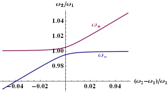
This diagram is what you will often see as "coupling diagram" in many, many respects. It does not matter so much if it happens between coupled oscillators or, for example, quantum systems. Why is this the case? Well, you couple harmonic oscillators. Harmonic oscillators model physical system pretty nicely and hence they are very often used. In turn, if you understand this worksheet (you might want to go through it again), you have understood a lot of other coupled systems as well! More on that in the background section after we have completely solved the worksheet!
Eigenfrequency analysis
The eigenfrequency analysis can by done by shortening the voltage supply. We directly arrive at the equations
\[\begin{eqnarray*} 0&=&\left(-\mathrm{i}\omega L_{1}+\frac{\mathrm{i}}{\omega C_{1}}\right)I_{1}\left(\omega\right)-\mathrm{i}\omega L_{c}I_{2}\left(\omega\right)\\0&=&\left(-\mathrm{i}\omega L_{2}+\frac{\mathrm{i}}{\omega C_{2}}\right)I_{2}\left(\omega\right)-\mathrm{i}\omega L_{c}I_{1}\left(\omega\right) \end{eqnarray*}\]
Now, multiply by \(\mathrm{i}\omega\) and each line with \(1/L_{i}\), we find in a matrix formulation
\[\begin{eqnarray*} 0&=&\left(\begin{array}{cc}\omega^{2}-\omega_{1}^{2} & \omega^{2}\kappa_{1}\\\omega^{2}\kappa_{2} & \omega^{2}-\omega_{2}^{2}\end{array}\right)\left(\begin{array}{c}
I_{1}\left(\omega\right)\\I_{2}\left(\omega\right)\end{array}\right)\ . \end{eqnarray*}\]
This yields the characteristic equation
\[\begin{eqnarray*} \left(\omega^{2}-\omega_{1}^{2}\right)\left(\omega^{2}-\omega_{2}^{2}\right)-\omega^{4}\kappa_{1}\kappa_{2}&=&0 \end{eqnarray*}\]
which is identical with our result for the infinite currents.
Note that we could in the same way arrive at a characteristic equation with losses in the circuits. We would find out that then the eigenfrequencies are indeed complex numbers accounting for the time-harmonic losses.
Background: Coupled Systems - Avoided Crossing, Hybridisation and all that
Two coupled systems form a combined system. If some energies of the original systems are comparable, the combined system may have drastically altered characteristics. We may exemplarily consider some coupled harmonic oscillator, see figure on the left: two equal masses attached to some walls with springs of equal modulus. If there was no coupling at all, both masses would oscillate at the same frequency.
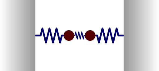 If, however, both masses are connected with a third spring, there will be two eigenmodes of the system: a symmetric and an antisymmetric oscillation of the two masses. Both oscillations will happen at different frequencies.
This detuning strongly depends on the coupling and is rather general. It can be observed in different fields of the natural sciences where we find different names for the phenomenon: avoided crossing for coupled two-level systems in quantum mechanics, hybridisation for interacting orbitals in chemistry, energy splitting in coupled mode theory and so on.
There is probably also a name for it in twin studies for supportively and destructively “coupled states”...
However, a more physical state-of-the-art example is “Direct Observation of Controlled Coupling in an Individual Quantum Dot Molecule” published in Physical Review Letters 94 (2005) by Krenner et. al. In the landmark paper, the authors report the anticrossing for coupled quantum dots and how it can be tuned by an external electric field.
Journal Page | arXiv | PDF


