![]() In this first tutorial we want to demonstrate the effects of perfectly matched layer boundary conditions and get to know the interactive FDTD toolbox.
In this first tutorial we want to demonstrate the effects of perfectly matched layer boundary conditions and get to know the interactive FDTD toolbox.
In FDTD-Simulations, it is extremely important to choose the right boundary conditions - three main types are of considerable importance: periodic boundaries, perfect reflecting ones and bounaries that absorb entirely - the perfectly matched layers. We want to take a look at the latter two in this tutorial. The reflection boundary condition means that an outwards propagating wave gets reflected at the boundary and propagates back into the computational domain. Before we get to know the perfectly matched layers, let us examine the situation in this case. This will also give us a feeling of how to use the program in general.
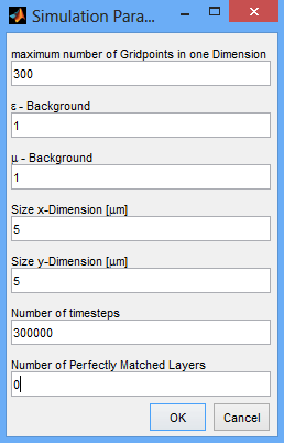
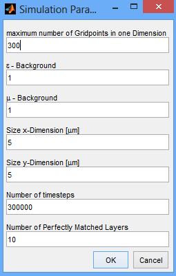
To start the iFDTD, we have to first start MATLAB and navigate into the folder, where the iFDTD is located. After that we may start it by typing "interactiveFDTD" in the command window. Now a dialog screen pops up - Here we define the general Parameters of our simulation:
maximum number of Gridpoints: defines our computational accuracy
ε and µ - Background: permittivity and permeability of the surrounding medium in our simulation
Size x and y Dimension: the lateral extensions of our computational domain
Number of timesteps: the number of time steps after the simulation quits - choose a smaller number if you want to save field values, then a matrix of size [spatial discretization x timesteps] will be generated. If you choose too much timesteps, you will probably run into memory issues.
Number of Perfectly Matched Layers: the number of perfectly matched layers - can be understood as the transition between mirror like - and transparent boundary conditions. For now, we choose "0" for reflecting boundaries.
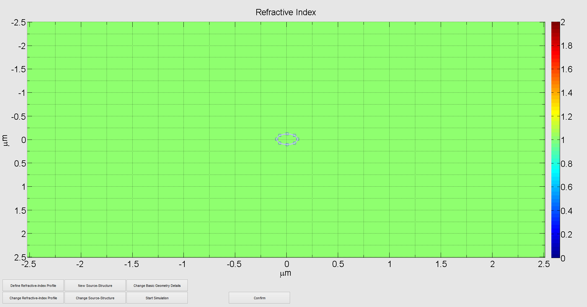
After the defnition of the general parameters for our simulation, the graphical user interface (GUI) appears to set up the simulation itself. Here we see seven buttons. With the help of them we can define and change sources and refractive index profiles.
Furthermore we can change the simulation parameters which we have set before. For our simulation we don't need a refractive index profile as we want to study the behavior of different boundary conditions.
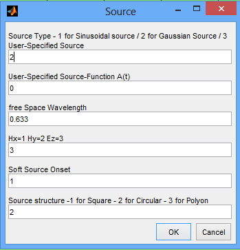
So we may simply add a source. To do so, please click on new source structure. An input interface like the one on the right appears. The different entries mean:
Source Type: type of the source - already implemented is a time-harmonic and a Gaussian source.
User-Specified Source Function A(t): This value only has a meaning if source type is "3" - Here you can define your own source function as Matlab Function handle, for example @(t) cos(omega*t)
free space Wavelength: defines the wavelength used for the source
Hx=1 Hy=2 Ez=3: excitation field component of the source
Soft Source Onset: Defines wether the source is hardly defined or with laterally gaussian shape
Source structure: shape of the source
After confirmation we are able to interactively define the source as depicted below:
For confirmation of the shape of the source we have to click confirm once again. If you want to change the source structure later on you press change source structure and redefine your source. You may as well define multiple sources to study interference effects.
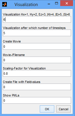
Now we have all defined to run a first simulation. Therefore we click the "Start Simulation" button. A new window appears where we have to specify how the calculations shall be presented to us. Here again we have different choices:
Visualization: defines which field component is visualized where |H| and |E| refer to the norm of the magnetic and electric field and |S| to the norm of the Poynting vector. Furthermore it also defines which field component is saved.
Visualization after which number of time steps: A lot of computational time is needed for visualization, so you can define a number after how many time steps the field is visualized.
Create Movie: enables you to save a movie if wanted which is generated while the simulation (Works only on 32-bit systems) - "1" for yes and "0" for no.
Movie-/Filename: If you want to save a movie and/or the field values, you can set the filename here.
Scaling Factor: Defines the scaling bar for visualization
Create File: "1" for yes "0" for no
Show PMLs: Enables you to show the defined number of PMLs which can be useful to see if the PML are working.
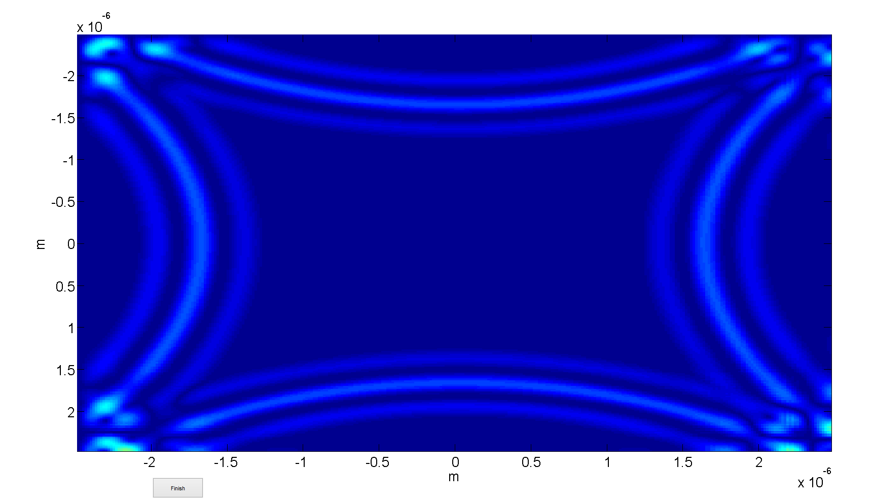
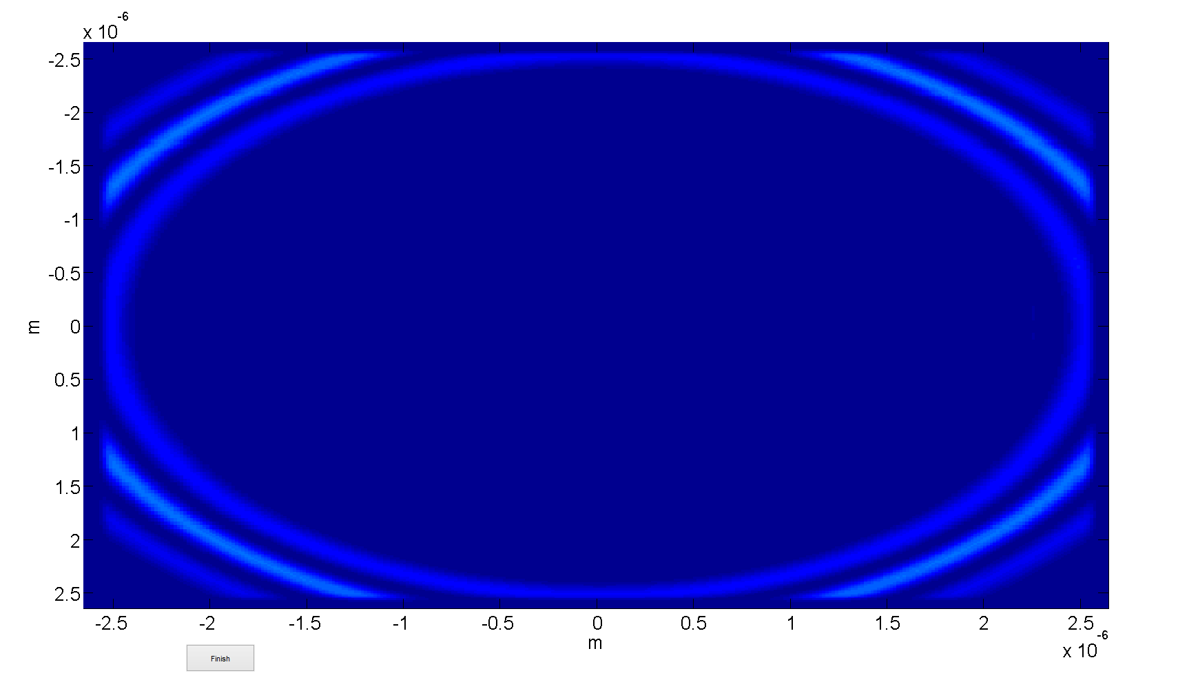
After confirmation, the simulation starts in a new window and the choosen field is visualized. The output for the values we used is shown below:
Reflecting boundary conditions: a radially outwards propagating wave gets reflected at the boundary.
Often, reflections into the physical domain of interest are rather unwanted. This is the case if we want to study a certain object subject to a well-defined excitation. In this situation, backreflections cause unwanted interference effects.
After confirmation we press start simulation again and the change the variable for "Show PMLs" from 0 to 1 in the visualization settings to show the PML's in the visualization. After confirmation the simulation starts again and we can observe the following output:
We now see that the pulse is propagating outwards - but now there is no reflection at the boundaries, the radiation gets absorbed in the PML-region, which is computationally equal to the transparent boundary condition.
Of course this is just a first rather "hello, world"-like example. Below you can see how PML's can be used in a more sophisticated situation to prefent back-scattering into the computational domain:
An example for perfectly matched layer boundary conditions in a simulation of the iFDTD: evanescent tunneling of a Gaussian beam through a prism. As desired, no backscattering at the boundaries can be observed.
2024 note: there appears to be some missing files here. Sorry for the incomplete example list!
