Tags: Image Charges / Dipole / Green's Function
![]() The Green's function can be used to find the electric field or electrostatic potential for arbitrary charge distributions. You will learn that the polarization of a dipole in front of a flat metallic surface enormously affects the overall field.
The Green's function can be used to find the electric field or electrostatic potential for arbitrary charge distributions. You will learn that the polarization of a dipole in front of a flat metallic surface enormously affects the overall field.
Problem Statement
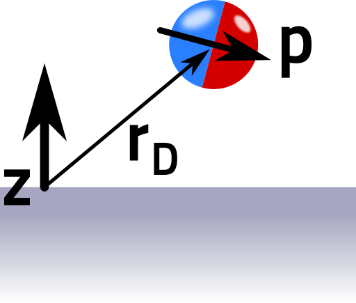
Use the Green's function to calculate the electrostatic potential 𝜙(r) for a dipole p at rD in front of a flat metallic surface terminated at z = 0.
Determine the main contributions to the potential for |rD| ≪ |r|.
Which contribution has a stronger fall-of: x- or z-polarization? Can you explain this in simple words?
Hints
What is the Green's function G(r,r') of a flat metallic surface? Remember the mirror charge technique (grounded metallic corner problem) and that the Green's function is basically just the field of a point charge at r'. Then,
\[\phi\left(\mathbf{r}\right)=\int G\left(\mathbf{r},\mathbf{r}^{\prime}\right)\rho\left(\mathbf{r}^{\prime}\right)dV^{\prime}\]
The charge distribution of a mathematical dipole is formally given by
\[\rho_{D}\left(\mathbf{r}\right)=-\mathbf{p}\cdot\nabla\delta\left(\mathbf{r}-\mathbf{r}_{D}\right)\]
A Taylor expansion can be a quite useful tool for approximations and also outlined in the dipole calculations.
Let us find the electric field for a dipole in front of a flat metallic surface!
The Electrostatic Potential
Let us write down the Green's function for the given system. Of course we know that for a single charge at
\[\mathbf{r}^{\prime} = \left(\begin{array}{c}x^{\prime}\\y^{\prime}\\z^{\prime}\end{array}\right)\ ,\]
the mirror charge would have to be placed at
\[\mathbf{r}_{m}^{\prime} = \left(\begin{array}{c}x^{\prime}\\y^{\prime}\\{\color{red}-}z^{\prime}\end{array}\right)\ .\]
Then, the Green's function is given by
\[G\left(\mathbf{r},\mathbf{r}^{\prime}\right) = \frac{1}{4\pi\varepsilon_{0}}\left(\frac{1}{\left|\mathbf{r}-\mathbf{r}^{\prime}\right|}-\frac{1}{\left|\mathbf{r}-\mathbf{r}_{m}^{\prime}\right|}\right)\ .\]
To find the electrostatic potential for the dipole, we have to use the charge distribution of it:
\[\rho_{D}\left(\mathbf{r}\right) = -\mathbf{p}\cdot\nabla\delta\left(\mathbf{r}-\mathbf{r}_{D}\right)\ .\]
We obtained this formula in "The Electric Field of a Dipole" , if you want to check the expression. So, we use the solution of the Poisson equation to formally find
\[\begin{eqnarray*} \phi\left(\mathbf{r}\right)&=&\int G\left(\mathbf{r},\mathbf{r}^{\prime}\right)\rho\left(\mathbf{r}^{\prime}\right)dV^{\prime}\\&=&-\mathbf{p}\cdot\int G\left(\mathbf{r},\mathbf{r}^{\prime}\right)\nabla_{\mathbf{r}^{\prime}}\delta\left(\mathbf{r}^{\prime}-\mathbf{r}_{D}\right)dV^{\prime}\\&=&\mathbf{p}\cdot\int\left[\nabla_{\mathbf{r}^{\prime}}G\left(\mathbf{r},\mathbf{r}^{\prime}\right)\right]\delta\left(\mathbf{r}^{\prime}-\mathbf{r}_{D}\right)dV^{\prime} \end{eqnarray*}\]
by partial integration. We now have to determine the gradient of the Green's function with respect to its second variable! First for the x component:
\[\begin{eqnarray*} \frac{\partial}{\partial x^{\prime}}G\left(\mathbf{r},\mathbf{r}^{\prime}\right)&=&\frac{1}{4\pi\varepsilon_{0}}\frac{\partial}{\partial x^{\prime}}\left(\frac{1}{\left|\mathbf{r}-\mathbf{r}^{\prime}\right|}-\frac{1}{\left|\mathbf{r}-\mathbf{r}_{m}^{\prime}\right|}\right)\\&=&\frac{1}{4\pi\varepsilon_{0}}\left(\frac{x-x^{\prime}}{\left|\mathbf{r}-\mathbf{r}^{\prime}\right|^{3}}-\frac{x-x^{\prime}}{\left|\mathbf{r}-\mathbf{r}_{m}^{\prime}\right|^{3}}\right) \end{eqnarray*}\]
and likewise for the y component. Note that we have used
\[\left|\mathbf{r}-\mathbf{r}^{\prime}\right|=\sqrt{\left(x-x^{\prime}\right)^{2}+\left(y-y^{\prime}\right)^{2}+\left(z-z^{\prime}\right)^{2}}\]
and that we have differentiated with respect to the second variable of the Green's function! Now for the z component:
\[\frac{\partial}{\partial z^{\prime}}G\left(\mathbf{r},\mathbf{r}^{\prime}\right) = \frac{1}{4\pi\varepsilon_{0}}\left(\frac{z-z^{\prime}}{\left|\mathbf{r}-\mathbf{r}^{\prime}\right|^{3}}{\color{red}+}\frac{z-z^{\prime}}{\left|\mathbf{r}-\mathbf{r}_{m}^{\prime}\right|^{3}}\right)\ .\]
We can already see the difference between both components of the Green's function's gradient: a sign change (denoted red). Now we put these components of the gradient into the solution of the Poisson equation and perform the integration:
\[\begin{eqnarray*} \phi\left(\mathbf{r}\right)&=&\mathbf{p}\cdot\int\left[\nabla_{\mathbf{r}^{\prime}}G\left(\mathbf{r},\mathbf{r}^{\prime}\right)\right]\delta\left(\mathbf{r}^{\prime}-\mathbf{r}_{D}\right)dV^{\prime}\\&=&\frac{1}{4\pi\varepsilon_{0}}\mathbf{p}\cdot\left(\begin{array}{c}\left(x-x_{D}\right)\left[\left|\mathbf{r}-\mathbf{r}_{D}\right|^{-3}-\left|\mathbf{r}-\mathbf{r}_{mD}\right|^{-3}\right]\\\left(y-y_{D}\right)\left[\left|\mathbf{r}-\mathbf{r}_{D}\right|^{-3}-\left|\mathbf{r}-\mathbf{r}_{mD}\right|^{-3}\right]\\\left(z-z_{D}^{\prime}\right)\left[\left|\mathbf{r}-\mathbf{r}_{D}\right|^{-3}+\left|\mathbf{r}-\mathbf{r}_{mD}\right|^{-3}\right]\end{array}\right)\ \text{with}\\\mathbf{r}_{mD}&=&\left(\begin{array}{c}x_{D}\\y_{D}\\{\color{red}-}z_{D}\end{array}\right)\ . \end{eqnarray*}\]
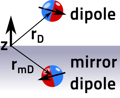 This is the solution of the electrostatic potential of a dipole in front of a flat metallic surface. We can directly see that it corresponds to a two-dipole-solution: a mirror-dipole appears at rmD (see figure).
Now let us try to understand the potential a little further
Taylor Expansion of the Potential
From a heuristic point of view it is clear that the dipole in z direction causes a mirror dipole pointing in the same direction. The x-polarization, parallel to the surface, corresponds to dipoles with opposite direction. Hence, the z-polarization should correspond to an overall dipolar field and the x polarization to a quadrupolar one. This is what we should find out.
Far away from the sources for |rD| ≪ |r|, we may Taylor-expand the denominators in the potential. The terms look rather similar, so we just have to calculate:
\[\frac{1}{\left|\mathbf{r}-\mathbf{r}_{D}\right|^{3}} \approx \frac{1}{\left|\mathbf{r}\right|^{3}}+\frac{3\mathbf{r}\cdot\mathbf{r}_{D}}{\left|\mathbf{r}\right|^{5}}\]
and analog for rmD, where the z component switches the sign. This is the important difference and we find
\[\begin{eqnarray*} \frac{1}{\left|\mathbf{r}-\mathbf{r}_{D}\right|^{3}}-\frac{1}{\left|\mathbf{r}-\mathbf{r}_{mD}\right|^{3}}&\approx&\frac{6z\, z_{D}}{\left|\mathbf{r}\right|^{5}}\ \text{and}\\\frac{1}{\left|\mathbf{r}-\mathbf{r}_{D}\right|^{3}}+\frac{1}{\left|\mathbf{r}-\mathbf{r}_{mD}\right|^{3}}&\approx&\frac{2}{\left|\mathbf{r}\right|^{3}}+\frac{6\left(x\, x_{D}+y\, y_{D}\right)}{\left|\mathbf{r}\right|^{5}}\ .\end{eqnarray*}\]
In this far-field approximation, the potential reads as
\[\phi\left(\mathbf{r}\right) \approx \frac{1}{4\pi\varepsilon_{0}}\mathbf{p}\cdot\left(\begin{array}{c}6x\, z\, z_{D}/\left|\mathbf{r}\right|^{5}\\6y\, z\, z_{D}/\left|\mathbf{r}\right|^{5}\\2z/\left|\mathbf{r}\right|^{3}+6z\left(x\, x_{D}+y\, y_{D}\right)/\left|\mathbf{r}\right|^{5}\end{array}\right)\]
and we have shown that the potential has a stronger fall-off behaviour for the x and y polarizations which goes effectively like \(\propto Q_{ij}x^{i}x^{j}/r^{5}\).
On the other hand the z polarization behaves as \(\propto p_{z}z/r^{3}\).
The figure below illustrates both cases:
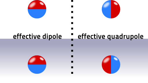
These potentials correspond to the quadrupolar and dipolar fields. We will find out later that oscillating dipoles radiate much faster than quadrupoles.
This is the reason why a dipole polarized parallel to the surface will basically heat the metal whereas the perpendicula polarization has a chance to escape the system. The polarization has thus a dramatic effect on the effectivity of emitter/metal-plate-systems.
Check again the multipole moment section for more information on multipole moments.
Background: Dipole Emitters in Front of Flat Metallic Surfaces
In this problem, we discuss the electrostatic dipole in the vicinity of a flat metal which is of huge interest both in applied and fundamental physics: think of a dipole antenna with a metal backplate or an emitting molecule. Of course such systems demand an understanding of full electrodynamics. The point is, however, that the main features will remain; x- and z-polarization will radiate differently.
It gets even more interesting if we do not have a perfect metal. Then, the electric field can penetrate the conductor and a closely placed dipole can excite surface waves as predicted by Sommerfeld more than one hundred years ago.
Even though this effect was not the explanation for long-range radio transmissions, the theory of Sommerfeld is still at the core of plasmonics, the field that deals with these so-called surface plasmon polaritons. For much more information on dipoles in front of flat metallic surfaces please have a look at Lukas Novotny's freely available book chapter on the topic.