Tags: Equations of Motion / Metric / Christoffel Symbols
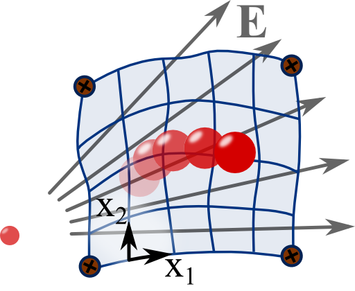
![]() The theoretical description of the movement of a particle in some curved 3D-space and the movement of it on a 2D-surface are equivalent. Both entities are described by a metric and the equation of motion is the geodesic equation. Further giving the particle a charge lets it further interact with an electric field. In this problem you can learn to derive the corresponding geodesic equation.
The theoretical description of the movement of a particle in some curved 3D-space and the movement of it on a 2D-surface are equivalent. Both entities are described by a metric and the equation of motion is the geodesic equation. Further giving the particle a charge lets it further interact with an electric field. In this problem you can learn to derive the corresponding geodesic equation.
Problem Statement
Consider the movement of a particle with charge q and mass m attached to a two-dimensional surface S in an external electrostatic field. Let us assume that the surface is described by the metric
\[g\left(\mathbf{r}\right)=g_{ij}\left(\mathbf{r}\right)dx^{i}dx^{j}\]
Using the definition of the Christoffel symbols,
\[\Gamma_{kl}^{i}\left(\mathbf{r}\right) \equiv \frac{1}{2}g^{im}\left(\mathbf{r}\right)\left(g_{mk,l}\left(\mathbf{r}\right)+g_{ml,k}\left(\mathbf{r}\right)-g_{kl,m}\left(\mathbf{r}\right)\right)\ ,\]
find an expression for the equation of motion of the particle. Compare your result to the equations of motion for a free particle in an electric field. Explain the meaning of the arising force terms.
Hints
As we know from theoretical mechanics, the equations of motion are given by the Euler-Lagrange equations
\[\frac{d}{dt}\frac{\partial L\left(\mathbf{r},\dot{\mathbf{r}}\right)}{\partial\dot{x}^{k}}-\frac{\partial L\left(\mathbf{r},\dot{\mathbf{r}}\right)}{\partial x^{k}} = 0\]
with the Lagrange function \(L=T-U\), kinetic minus potential energy. Given that the motion is restricted to the surface \(S\) described by the metric \(g\left(\mathbf{r}\right)\), what do you think is an appropriate expression for the kinetic energy?
Ok, let us find the geodesic movement of charge on a surface with electric field! We will find a close encounter to general relativity!
The Lagrange Function on the Surface
To find the solution of the problem we first write down the Lagrange function
\[\begin{eqnarray*}L\left(\mathbf{r},\dot{\mathbf{r}}\right) & =& T-U\\& = &\frac{m}{2}\dot{\mathbf{r}}^{2}-q\phi\left(\mathbf{r}\right)\\& = &\frac{m}{2}g_{ij}\left(\mathbf{r}\right)\dot{x}^{i}\dot{x}^{j}-q\phi\left(\mathbf{r}\right)\ .\end{eqnarray*}\]
But let us think about this representation and the concepts behind it a little. First of all, it is important to note that the coordinate \(\mathbf{r}\) of the particle lies in the surface \(S\) - there is no need to consider the embedding space. This also considers the velocity vector \(\dot{\mathbf{r}}\) of the particle. It always has to be part of the tangent space of the surface. If this was not the case, the charge could somehow escape it. Thus, we can measure its length using the metric of the surface as we did it in the Lagrange function.
In fact, since the surface is just a two-dimensional entity, the same holds for our problem. Only if we wanted to calculate the position and velocity of the particle in an embedding space, say \(\mathbb{R}^{3}\), we would have to find a function \(\varphi:\ S\rightarrow\mathbb{R}^{3}\) mapping \(\mathbf{r}\in S\rightarrow\mathbf{r}^{\prime}\in\mathbb{R}^{3}\).
The maybe astonishing fact is that we can calculate everything using the coordinates of the surface. This is conceptually linked to Gauss's Theorema Egregrium. It says that you can measure the curvature of a surface only considering local quantities of it - lengths and angles, hence, the metric.
Calculating the Equations of Motion
Now we are sure that our description is physically meaningful and can proceed to finally use the Euler-Lagrange equations
\[\frac{d}{dt}\frac{\partial L\left(\mathbf{r},\dot{\mathbf{r}}\right)}{\partial\dot{x}^{k}}-\frac{\partial L\left(\mathbf{r},\dot{\mathbf{r}}\right)}{\partial x^{k}} = 0\ .\]
We compute
\[\frac{\partial L\left(\mathbf{r},\dot{\mathbf{r}}\right)}{\partial x^{k}} = \frac{m}{2}g_{ij,k}\left(\mathbf{r}\right)\dot{x}^{i}\dot{x}^{j}-q\phi_{,k}\left(\mathbf{r}\right)\]
and the “generalized impulse”
\[\begin{eqnarray*}\frac{\partial L\left(\mathbf{r},\dot{\mathbf{r}}\right)}{\partial\dot{x}^{k}}&=&\frac{m}{2}\left(g_{ij}\left(\mathbf{r}\right)\dot{x}^{i}\delta_{k}^{j}+g_{ij}\left(\mathbf{r}\right)\delta_{k}^{i}\dot{x}^{j}\right)\\&=&\frac{m}{2}\left(g_{ik}\left(\mathbf{r}\right)\dot{x}^{i}+g_{kj}\left(\mathbf{r}\right)\dot{x}^{j}\right)\ .\end{eqnarray*}\]
Note again that in the first equation the derivative of the electrostatic potential \(\phi\) is with respect to the local coordinates of the surface. Furthermore, the metric is symmetric, \(g_{ij}\left(\mathbf{r}\right)=g_{ji}\left(\mathbf{r}\right)\). So, we could write the generalized impulse in a more compact form. Here, however, it is beneficial to maintain the current form to incorporate the Christoffel symbols later on.
Now, we have to derive the latter equation with respect to the time:
\[\begin{eqnarray*}\frac{d}{dt}\frac{\partial L\left(\mathbf{r},\dot{\mathbf{r}}\right)}{\partial\dot{x}^{k}}&=&\frac{d}{dt}\frac{m}{2}\left(g_{ik}\left(\mathbf{r}\right)\dot{x}^{i}+g_{kj}\left(\mathbf{r}\right)\dot{x}^{j}\right)\\&=&\frac{m}{2}\left(g_{ik}\left(\mathbf{r}\right)\ddot{x}^{i}+g_{ik,l}\left(\mathbf{r}\right)\dot{x}^{i}\dot{x}^{l}+g_{kj}\left(\mathbf{r}\right)\ddot{x}^{j}+g_{kj,l}\left(\mathbf{r}\right)\dot{x}^{j}\dot{x}^{l}\right)\\&=&m\ddot{x}_{k}+\frac{m}{2}\left(g_{ik,l}\left(\mathbf{r}\right)\dot{x}^{i}\dot{x}^{l}+g_{kj,l}\left(\mathbf{r}\right)\dot{x}^{j}\dot{x}^{l}\right)\ .\end{eqnarray*}\]
Now employing the Euler-Lagrange equations we find
\[\begin{eqnarray*}0&=&\frac{d}{dt}\frac{\partial L\left(\mathbf{r},\dot{\mathbf{r}}\right)}{\partial\dot{x}^{k}}-\frac{\partial L\left(\mathbf{r},\dot{\mathbf{r}}\right)}{\partial\dot{x}^{k}}\\&=&m\ddot{x}_{k}+\frac{m}{2}\left(g_{ik,l}\left(\mathbf{r}\right)\dot{x}^{i}\dot{x}^{l}+g_{kj,l}\left(\mathbf{r}\right)\dot{x}^{j}\dot{x}^{l}\right)\\& &-\frac{m}{2}g_{ij,k}\left(\mathbf{r}\right)\dot{x}^{i}\dot{x}^{j}+q\phi_{,k}\left(\mathbf{r}\right)\ .\end{eqnarray*}\]
So, how can we get an expression in the Christoffel symbols? If we multiply (summation!) the recent equation with \(g^{nk}\left(\mathbf{r}\right)\), which is the inverse of the metric, \(g^{ab}g_{bc}=\delta_{c}^{a}\), we find
\[\begin{eqnarray*}0&=&m\ddot{x}^{n}+\frac{m}{2}g^{nk}\left(\mathbf{r}\right)\left(g_{ik,l}\left(\mathbf{r}\right)+g_{ki,l}\left(\mathbf{r}\right)-g_{il,k}\left(\mathbf{r}\right)\right)\dot{x}^{i}\dot{x}^{l}+qg^{nk}\left(\mathbf{r}\right)\phi_{,k}\left(\mathbf{r}\right)\ \text{, so}\\0&=&m\ddot{x}^{n}+m\Gamma_{il}^{n}\left(\mathbf{r}\right)\dot{x}^{i}\dot{x}^{l}+q\phi^{,k}\left(\mathbf{r}\right)\ .\end{eqnarray*}\]
Now, how does this compare to flat space? In the absence of a magnetic field, the Lorentz force is given by \(m\ddot{\mathbf{r}}=q\mathbf{E}\left(\mathbf{r}\right)\). This corresponds to the term \(\phi\)-term since \(\mathbf{E}\left(\mathbf{r}\right)=-\nabla\phi=-\phi^{,k}\mathbf{e}_{k}\). For a vanishing electric field we just have a geodesic motion along the surface. The Christoffel symbols thus represent the constraint force attaching the particle to the surface.
Relativistic Notation
Note that in this problem it is helpful to use the condensed Einstein notation for which we leave out the summation symbol if an index appears both up- and downwards of a quantity:\[\sum_{i}u^{i}v_{i} = u^{i}v_{i}=g_{ij}\left(\mathbf{r}\right)u^{i}v^{i}\ .\]As we can see, indices can be “moved” with the metric - lower und upper indices correspond to a representation in cotangent and tangent space, respectively. The length of a vector can be calculated using \(g_{ij}\): \(\mathbf{u}^{2}=g_{ij}u^{i}u^{j}\equiv g\left(\mathbf{u},\mathbf{u}\right)\). For a surface in a cartesian (flat) x-y-plane we would simply have \(g_{ij}=\delta_{ij}\) and the squared length of a vector would be just \(\mathbf{u}^{2}=u_{x}^{2}+u_{y}^{2}\).
Furthermore, partial derivatives can also be denoted by a comma, \(\partial f\left(x\right)/\partial x=\partial_{x}f\left(x\right)=f_{,x}\left(x\right)\). See also our section on relativistic electrodynamics for more in-depth informattion.
Background: Geodesic Motion in General Relativity
In the case of a vanishing electric field we will derive a very general and important result. It explains the motion of a particle not only on surfaces but holds for motions on “generalized surfaces” called manifolds with a given metric \(g_{\mu\nu}\left(x^{\alpha}\right)\). The equation can also be derived from the requirement of the minimum of the length
\[L = \int_a^b \sqrt{g_{\mu\nu}\left(x^{\alpha}\left(\tau\right)\right)\frac{dx^{\mu}}{d\tau}\frac{dx^{\nu}}{d\tau}}d\tau\]
of a curve \(x^{\alpha}\left(\tau\right)\) connecting two points on that manifold. Such a shortest path is called a geodesic and the equation we will derive consequentially termed geodesic equation.
In general relativity, the metric itself represents the gravitational field. However, it is not the metric of just space but also includes time components. Roughly speaking, all kinds of matter and energy affect the metric as described by the Einstein field equations. In our problem we assumed that the mass or velocity of our charge does not influence the surface, i.e. the metric. In general relativity this is an approximation - the geodesic motion is assumed to not influence the metric. The geodesic equation thus describes the movement of a test particle through spacetime.
Electromagnetic fields itself can be the source of gravitation since they contain energy. This can also be incorporated into general relativity. The corresponding theory is called Einstein-Maxwell theory. In our problem, the metric is given ad-hoc and not influenced by the electrostatic field.