The Electric Field of two Point Charges

Sometimes it happens that a thing is more than the sum of its parts. What about two charges? Can their respective electric field behave fundamentally different in some way than just a single charge? In this problem you will learn about two main concepts in electromagnetics - the superposition principle and the dipole.

Problem Statement

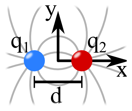
Two electric charges, q₁ = +q and q₂ = -q, are placed on the x axis separated by a distance d.

Using Coulomb's law and the superposition principle, what is the magnitude and direction of the electric field on the y axis?

What happens if both charges are equal? Draw a schematic of the fields for both cases in the x,y-plane in a field line plot.

Background: The Superposition Principle

The superposition principle plays a mayor role in (linear) electrodynamics. It allows the calculation of electromagnetic fields with arbitrary charge distributions.
One configuration is of particular interest - two separated point charges of opposite charge. In the limit of vanishing separation, it is called dipole.

Its field fundamentally differs from that of just a single charge even though it is just the sum of the charge. The dipole as a concept is extremely important throughout electrodynamics.

It is applied for example explaining the emission of electromagnetic radiation or as a model for molecules, see The Precessing Dipole Molecule. This problem will guide us in this direction.

Hints

What is Coulomb's law again and how do we know the electric field of a point charge from it? If you do not remember, you can lookup the corresponding question.

Can you explain the superposition principle?

Alright, let us find the electric field of two point charges!

Solution

The superposition principle states that the field of a charge configuration is given by the sum of the fields of the respective charges,

\[\begin{eqnarray*}\mathbf{E}\left(\mathbf{r}\right) & = & \frac{1}{4\pi\epsilon_{0}} \sum_{i}q_{i} \frac{\mathbf{r}-\mathbf{r}_{i}}{ \left|\mathbf{r}- \mathbf{r}_{i}\right|^{3}}\ .\end{eqnarray*}\]

Naturally the summation contains all charges, indexed by the i. Using this principle we can calculate the fields for any charge configuration. Here we want to find some insight for the easiest case possible, two charges of opposite and equal charge.

 

Opposite Charges

Let us first consider the case of opposite charges. For the given problem we have \(\mathbf{r}_{1} =-d/2\, \mathbf{e}_{x}\) and \(\mathbf{r}_{2 = d/2\,\mathbf{e}_{x}\).

So the charges lie on the \(x\) axis with a separation \(d\). Remember that \(\mathbf{e}_{x}\) is the unit vector in \(x\) direction. The electric field is then given by

\[\begin{eqnarray*}\mathbf{E}\left(\mathbf{r}\right) & = & \frac{1}{4\pi\epsilon_{0}}\left \{ q_{1} \frac{\mathbf{r}-\mathbf{r}_{1}}{\left|\mathbf{r}-\mathbf{r}_{1}\right|^{3}}+q_{2} \frac{\mathbf{r}- \mathbf{r}_{2}}{\left|\mathbf{r}-\mathbf{r}_{2} \right|^{3}}\right\} \\& = & \frac{q}{4\pi\epsilon_{0}}\left\{ \frac{ \left(x-d/2\right)\mathbf{e}_{x}+y\mathbf{e}_{y}+z\mathbf{e}_{z}}{\left[\left(x-d/2\right)^{2}+y^{2}+z^{2}\right]^{3/2}}-\frac{\left(x+d/2\right) \mathbf{e}_{x}+y\mathbf{e}_{y}+ z \mathbf{e}_{z}}{\left|\left(x+d/2\right)^{2}+y^{2}+z^{2}\right|^{3/2}}\right\} \ .\end{eqnarray*}\]

Remembering that the norm of a vector is given by \(\left|a\mathbf{e}_{x}+b\mathbf{e}_{y}+c\mathbf{e}_{z}\right|=\sqrt{a^{2}+b^{2}+c^{2}}\).

For the given problem, the magnitude and direction of the field on the \(y\) axis was asked for. To figure out both, we first calculate the whole field:

\[\begin{eqnarray*}\mathbf{E}\left(x=0,y,z=0\right) & = & \frac{q}{4\pi\epsilon_{0}}\left\{ \frac{-d/2\,\mathbf{e}_{x}+y\mathbf{e}_{y}}{\left[\left(d/2\right)^{2}+y^{2}\right]^{3/2}}-\frac{d/2\,\mathbf{e}_{x}+ y\mathbf{e}_{y}}{\left|\left(d/2\right)^{2}+y^{2}\right|^{3/2}}\right\} \\ & = & \frac{q}{4\pi \epsilon_{0}}\left\{ \frac{-d\,\mathbf{e}_{x}}{ \left[\left(d/2\right)^{2}+y^{2}\right]^{3/2}}\right\} \ .\end{eqnarray*}\]

We see that the electric field has only a component in x direction. Because of the symmetric choice of the coordinate system we could have guessed this in the first place.

The magnitude is given by the norm of the electric field,

\[\begin{eqnarray*} \left|\mathbf{E} \left(x=0,y,z=0\right)\right| & = & \frac{q}{4\pi\epsilon_{0}}\frac{d}{\left[ \left(d/2\right)^{2}+y^{2} \right]^{3/2}}\\ & = & \frac{q}{4\pi \epsilon_{0}}\frac{1}{d^{2}} \frac{1}{\left[\left(1/2\right)^{2}+ \left(y/d\right)^{2}\right]^{3/2}} \end{eqnarray*}\]

The magnitude of the field on the \(y\) axis is a monotonic decreasing function for positive \(y\), falling for large \(y\) as \(1/y^{3}\). So maybe these two charges are just more than their sum! In the limit of $d\rightarrow0$ with \(p=q\cdot d=\mathrm{const}\), this charge distribution is called a dipole for which we just calculated the large distance behavior. Let us now consider the case of equal charges.

Equal Charges

If the two charges are equal to \(q\), we find the electric field again as a superposition of both charges:

\[\begin{eqnarray*} \mathbf{E}\left(x=0,y,z=0\right) & = & \frac{q}{4\pi\epsilon_{0}}\left\{ \frac{-d/2\,\mathbf{e}_{x}+y \mathbf{e}_{y}}{ \left[\left(d/2\right)^{2}+y^{2} \right]^{3/2}}+\frac{d/2\,\mathbf{e}_{x}+ y\mathbf{e}_{y}}{\left|\left(d/2\right)^{2}+y^{2} \right|^{3/2}}\right\} \\ & = & \frac{2q}{4\pi\epsilon_{0}}\left\{ \frac{y\,\mathbf{e}_{y}}{\left[ \left(d/2\right)^{2}+y^{2} \right]^{3/2}}\right\} \ .\end{eqnarray*}\]

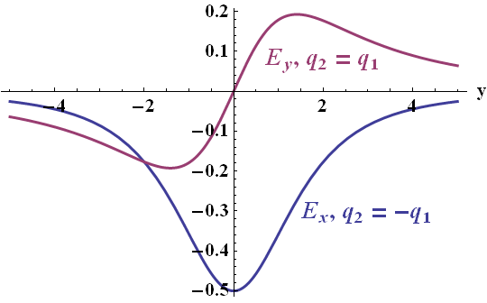
The direction of the field is in this case always parallel to the y axis but changing sign at y = 0. Its magnitude is given by

\[\begin{eqnarray*} \left|\mathbf{E}\left(x=0,y,z=0\right)\right| & = & \frac{2q}{4\pi\epsilon_{0}}\frac{\left|y\right|}{\left[\left(d/2\right)^{2}+y^{2}\right]^{3/2}}\\ & = & \frac{2q}{4\pi\epsilon_{0}}\frac{1}{y^{2}}\frac{1}{ \left[\left(d/2y\right)^{2}+1\right]^{3/2}}\ . \end{eqnarray*}\]

We find that for equal charges the magnitude of the electric field decreases for large y as the field of a particle with charge \(2q\). On the right you can see the field along the y axis, i.e. the nonvanishing field components in the case of opposite and equal charges.

 

Field Line Plot

A good way to visualize a vector field is by using a field line plot. Frankly speaking you take one point in space, evaluate the direction of the vector field at this point and go a certain distance in that direction. Then you connect both points, e.g. by an arrow and repeat the procedure from the new point.

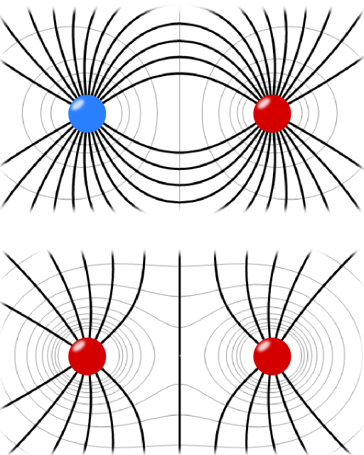
As you can imagine this can get a quite tedious procedure if you want to do it precisely. Most of the time it is much better to just make a brief sketch that contains the basic information. This is the case if you want to explain something about the field to a colleague.

However, if you need nice graphics, it is much better to let somebody do it for you, for example a computer. Most of the modern computer algebra systems can handle this task. I prefer Mathematica and made some minor changes to the code available from a Wolfram demonstration project to produce some data for the field line plot on the right. I have to excuse myself at this point for being too lazy to fill in the arrows indicating the field direction from positive to negative charges.

But hey, maybe you are more patient! It is always nice to figure out how to visualize physical contexts for for others!