Tags: Spectrum / Heaviside function
After we have understood the Fourier Transformation of the Heaviside Function, we can now apply our knowledge to the spectrum of a pulsed electric field. This can be done by the Fourier transform of a Heaviside function with underlying oscillating electric field.
Problem Statement
We have a rectangular shaped pulse with central frequency (\omega_0) given by:
[E(t)=\cos(\omega_0t)\Theta\left(1-\left|\frac{t}{a}\right|\right).]
Here the Heaviside-function (\Theta(x)) is used, which is defined as:
[\begin{eqnarray}\Theta(x)=\left{\begin{array}{ccc}1 &\mathrm{if} & x>0 \0 &\mathrm{else} &\end{array}\right.\end{eqnarray}]
Calculate the spectrum of the pulse (\ {E}(\omega)) using Fourier-Transformation.

Hints
The Fourier-Transformation in photonics s is given by:
\[E\left(\mathbf{r},t\right)=\int\limits_{-\infty}^{\infty}{d\omega}{\overline{E}\left(\mathbf{r},\omega\right)e^{-i\omega t}}\;\mathrm{and\;}E\left(\ {r},\omega\right)=\frac{1}{2\pi}\int\limits _{-\infty}^{\infty}{dt}{\overline{E}\left(\mathbf{r},\omega\right)e^{i\omega t}}\]
To simplify the integral use substitution, the exponential expression for \(\cos(\omega_{0}t)\).
Ok, let us find the spectrum of a rectangular pulse!
Direct integration using definition of Heaviside function
Since we are not interested in the space-coordinate we will drop the \(\mathbf{r}\) in the argument of the eletric field.
\[\overline{E}(\omega)=\frac{1}{2\pi}\int\limits_{-\infty}^{\infty}{dt}{e^{i\omega t}\cos(\omega_{0}t)\Theta\left(1-\left|\frac{t}{a}\right|\right)}\]
To simplify the integration of the Heaviside-function use variable-substitution:
\[z=\frac{t}{a}\rightarrow\frac{dz}{dt}=\frac{1}{a}\rightarrow dt=a\cdot dz\]
So we get the new equation:
\[\overline{E}(\omega)=\frac{a}{2\pi}\int\limits _{-\infty}^{\infty}dze^{i\omega az}\cos(\omega_{0}az)\Theta\left(1-\left|z\right|\right)\]
Use the Euler-identity for the \(\cos\)-function: \[\cos\left(x\right)=\frac{e^{ix}+e^{-ix}}{2}\]
\begin{eqnarray*} \overline{E}(\omega)&=&\frac{a}{4\pi}\int\limits _{-\infty}^{\infty}dze^{i\omega az}\left(e^{i\omega_{0}az}+e^{-i\omega_{0}az}\right)\Theta\left(1-\left|z\right|\right)\\&=&\frac{a}{2\pi}\int\limits _{-\infty}^{\infty}dz\left(e^{i\left(\omega+\omega_{0}\right)az}+e^{i\left(\omega-\omega_{0}\right)az}\right)\Theta\left(1-\left|z\right|\right) \end{eqnarray*}
Here you must use partial integration which is defined by:
\[\int{u'v}=uv-\int{uv'}\]
where \(u'=\left(e^{i\left(\omega+\omega_{0}\right)az}+e^{i\left(\omega-\omega_{0}\right)az}\right)\) and \(v=\Theta\left(1-\left|z\right|\right)\). We get \(u\) by integrating \(u'\), which is easy. We can simply write:
\[u=\frac{e^{i\left(\omega+\omega_{0}\right)az}}{i\left(\omega+\omega_{0}\right)a}+\frac{e^{i\left(\omega-\omega_{0}\right)az}}{i\left(\omega-\omega_{0}\right)a}.\]
The derivative of the Heaviside-function is the delta-distribution. You can derive it by partial integration:
\begin{eqnarray*} \Theta'\left[f\left(x\right)\right]&=&\Theta\left[f\left(x\right)\right]-\Theta\left[f'\left(x\right)\right]\\&=&-\int\limits _{0}^{\infty}dxf'\left(x\right)\\&=&-\left[f\left(\infty\right)-f\left(0\right)\right]\\&=&f\left(0\right)=\delta_{0}\left[f\left(x\right)\right] \end{eqnarray*}
So, we get:
\[v'=\delta(1+z)-\delta(1-z)\]
Now we can write:
\begin{eqnarray*}\overline{E}(\omega)&=&\frac{a}{4\pi}\left[\left(\frac{e^{i\left(\omega+\omega_{0}\right)az}}{i\left(\omega+\omega_{0}\right)a}+\frac{e^{i\left(\omega-\omega_{0}\right)az}}{i\left(\omega-\omega_{0}\right)a}\right)\Theta\left(1-\left|z\right|\right)\right]_{-\infty}^{\infty}\\&-&\frac{a}{4\pi}\left[\int\limits _{-\infty}^{\infty}dz\left(\frac{e^{i\left(\omega+\omega_{0}\right)az}}{i\left(\omega+\omega_{0}\right)a}+\frac{e^{i\left(\omega-\omega_{0}\right)az}}{i\left(\omega-\omega_{0}\right)a}\right)\left(\delta\left(1+z\right)-\delta\left(1-z\right)\right)\right]\\&=&\frac{a}{4\pi}\int\limits _{-\infty}^{\infty}dz\frac{e^{i\left(\omega+\omega_{0}\right)az}}{i\left(\omega+\omega_{0}\right)a}\delta\left(1-z\right)+\int\limits _{-\infty}^{\infty}dz\frac{e^{i\left(\omega-\omega_{0}\right)az}}{i\left(\omega-\omega_{0}\right)a}\delta\left(1-z\right)\\&-&\frac{a}{4\pi}\left[\int\limits _{-\infty}^{\infty}dz\frac{e^{i\left(\omega+\omega_{0}\right)az}}{i\left(\omega+\omega_{0}\right)a}\delta\left(1+z\right)+\int\limits _{-\infty}^{\infty}dz\frac{e^{i\left(\omega-\omega_{0}\right)az}}{i\left(\omega-\omega_{0}\right)a}\delta\left(1+z\right)\right]\\&=&\frac{a}{4\pi}\left[\frac{e^{i\left(\omega+\omega_{0}\right)a}}{i\left(\omega+\omega_{0}\right)a}+\frac{e^{i\left(\omega-\omega_{0}\right)a}}{i\left(\omega-\omega_{0}\right)a}-\frac{e^{-i\left(\omega+\omega_{0}\right)a}}{i\left(\omega+\omega_{0}\right)a}-\frac{e^{-i\left(\omega-\omega_{0}\right)a}}{i\left(\omega-\omega_{0}\right)a}\right]\\&=&\frac{1}{2\pi}\left[\frac{\sin\left[\left(\omega+\omega_{0}\right)a\right]}{\omega+\omega_{0}}+\frac{\sin\left[\left(\omega-\omega_{0}\right)a\right]}{\omega-\omega_{0}}\right] \end{eqnarray*}
Integration after changing integral limits
The same result can be obtained much easier by changing the integration limits imposed by the Heaviside-function:
\[\begin{eqnarray*}\ {\overline{E}}(\omega)&=&\frac{1}{2\pi}\int\limits_{-\infty}^{\infty}dte^{i\omega t}\cos(\omega_{0}t)\Theta\left(1-\left|\frac{t}{a}\right|\right)\\&=&\frac{1}{2\pi}\int\limits_{-a}^{a}dte^{i\omega t}\cos(\omega_{0}t)\\&=&\frac{1}{4\pi}\int\limits _{-a}^{a}dt\left\{ e^{i(\omega+\omega_{0})t}+e^{-i(\omega-\omega_{0})t}\right\} \\&=&\frac{1}{4\pi}\left[\frac{e^{i(\omega+\omega_{0})t}}{i\left(\omega+\omega_{0}\right)}+\frac{e^{i(\omega-\omega_{0})t}}{i\left(\omega-\omega_{0}\right)}\right]_{-a}^{a} \end{eqnarray*}\]
This looks similar to the integral above. The result is:
\[ \overline{E}(\omega)=\frac{1}{2\pi}\left[\frac{\sin\left[\left(\omega+\omega_{0}\right)a\right]}{\omega+\omega_{0}}+\frac{\sin\left[\left(\omega-\omega_{0}\right)a\right]}{\omega-\omega_{0}}\right]\]
Solving by using the translation rule for Fourier-Transformation
A third method to solve for the spectrum is by using the translation rule for Fourier-Transformation. Once we have the Fourier Transform of the rectangular function:
\[\frac{1}{2\pi}\int\limits _{-\infty}^{\infty}dte^{-i\omega t}\Theta\left(1-\left|\frac{t}{a}\right|\right)=\frac{a}{\pi}\text{sinc}(a\omega)\]
and the exponential expansion of the \(\cos(\omega_{0}t)\):
\[\cos(\omega_{0}t)=\frac{1}{2}(e^{i\omega_{0}t}+e^{-i\omega_{0}t})\]
we get by using the shift theorem:
\[FT=\frac{a}{2\pi}\left(\text{sinc}(a(\omega-\omega_{0}))+\text{sinc}(a(\omega+\omega_{0}))\right)\]
Illustration of the results
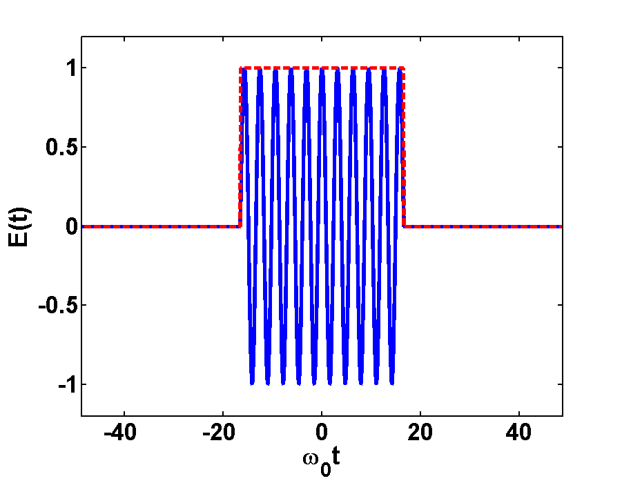
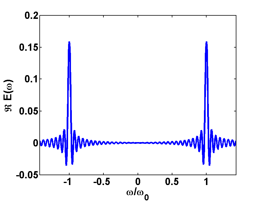
In Fig.1 and Fig.2 the time- and Fourier-spectrum of a light pulse is illustrated. Fig.1a shows a very short pulse, here we took a plane wave and cut out a small piece in time domain. If we transform this short pulse to Fourier domain, then we will get a broad frequency-spectrum, as it is shown in Fig.1b. Here we take in account the FWHM of the peaks at \(\frac{\omega}{\omega_{0}}=\pm1
\).
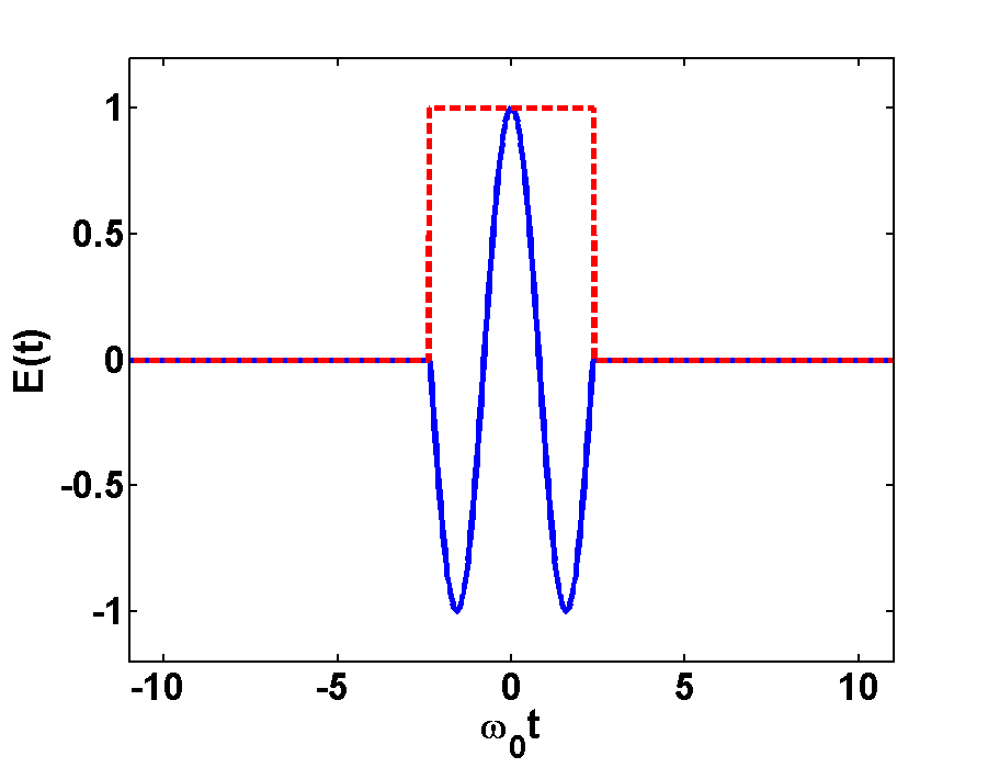
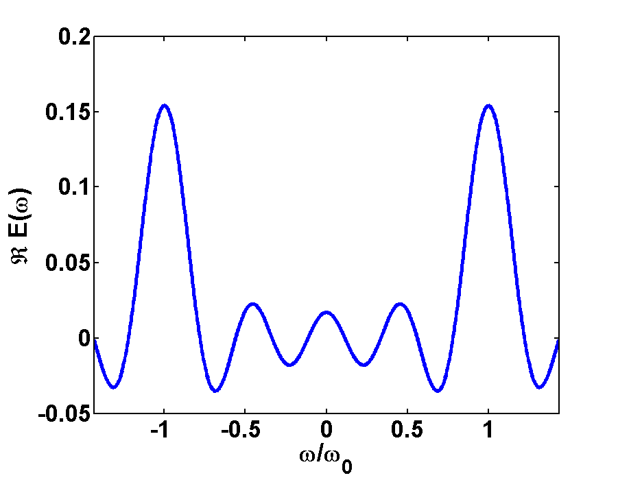
Fig.2a shows a long pulse, where a piece containing some more wavelengths was taken out. If we transform this long pulse to Fourier domain we will get a narrow frequency-spectrum, as it is shown in Fig.1b. Here we see two narrow peaks of the sinc functions at \(\frac{\omega}{\omega_{0}}=\pm1\)and therefore more information about this pulse than about the short pulse.