Fabry-Perot Resonances in a Transmission Line

One of the most important concepts in optics are Fabry-Perot resonances of certain cavities. Nevertheless, we can understand this resonance phenomenon on the basis of wave propagation in transmission lines! You can also find out how this principle is used in nanophotonics.

Problem Statement

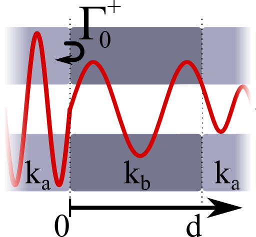A transmission line a is intercepted at x = 0 by another transmission line b of length d. Transmission line b exhibits a different characteristic impedance than a.

The voltage reflection coefficient at x = 0 shall be given by

\[\Gamma_{0}^{+}=\left|\Gamma_{0}^{+}\right|e^{\mathrm{i}\phi_{r}}\ .\]

Show that the overall transmission coefficient for this configuration is given by

Here, the \(T_{0/d}^{+}\) are the transmission coefficients at x = 0 and x = d, respectively.

\(k_{b}=k_{b}^{\prime}+\mathrm{i}k_{b}^{\prime\prime}\) is the wavenumber of the transmission line \(b\).

For a certain incoming power \(P_{i}\left(x=0\right)\), find the total transmitted power through the system at x = d

Verify that if the intercepting line is lossless, the transmitted power is maximal if the Fabry-Perot resonance condition

\[\begin{eqnarray*} 2k_{b}^{\prime}d+2\phi_{r}&=&2\pi n \end{eqnarray*}\]

holds. Derive a modified resonance condition if losses are present, i.e. \(k_{b}^{\prime\prime}>0\).

Hints

The transmission coefficient can be seen as sum over all possible transmission scenarios.

So, which reflection coefficients are needed and how are they related to \(\Gamma_{0}^{+}\)?

The transmitted power is given by \(P_{t}=\left|T\right|^{2}P_{i}\).

Ok, let's jump directly into the solution for the Fabry Perot line transmission coefficient!

Solution

To find the transmission coefficient we have to first know understand the reflection inside of transmission line \(b\). After this we will calculate the transmission coefficient by a summation over all possible scenarios leading to an overall transmission. Finally, we will see that a maximum transmission is linked to the Fabry-Perot resonance condition.

Calculating the needed Reflection Coefficients

First of all we have to answer how the reflection coefficient looks like if we reflect at some point \(x^{\prime}\) and not at the origin. A decomposition in forward and backwards propagating waves in a transmission line \(a\) is given by (see again Impedance Matching of Transmission Lines and Oscillator Circuits for more details)\[\begin{eqnarray*} U\left(x\right)&=&U_{a}^{+}\left(e^{\mathrm{i}k_{a}x}+\Gamma e^{-\mathrm{i}k_{a}x}\right)\ ,\\I\left(x\right)&=&\frac{U_{a}^{+}}{Z_{a}}\left(e^{\mathrm{i}k_{a}x}-\Gamma e^{-\mathrm{i}k_{a}x}\right) \end{eqnarray*}\]where we assume a reflection backwards. In another transmission line, say \(b\), we only consider outwards going waves and find by continuity:\[\begin{eqnarray*} \Gamma_{x^{\prime}}&=&\frac{Z_{b}-Z_{a}}{Z_{b}+Z_{a}}e^{\mathrm{i}2k_{a}x^{\prime}}=\Gamma_{0}^{+}e^{\mathrm{i}2k_{a}x^{\prime}}\ . \end{eqnarray*}\]Here, we may call \(\Gamma_{0}^{+}\) the reflection coefficient in positive direction at the origin. For the propagation in negative direction we have to make the same calculation. Keeping in mind that \(Z_{a}=-U_{a}^{-}/I_{a}^{-}\), we find that there is no sign change for the reflection forwards, \(\Gamma_{x^{\prime}}^{\pm}=\Gamma_{x^{\prime}}\). For our specific problem we need two reflection coefficients, both from medium \(b\) to \(a\):\[\begin{eqnarray*} \Gamma_{d}^{+}&=&\frac{Z_{a}-Z_{b}}{Z_{a}+Z_{b}}e^{\mathrm{i}2k_{b}d}=-\Gamma_{0}^{+}e^{\mathrm{i}2k_{b}d}\ .\\\Gamma_{0}^{-}&=&\frac{Z_{a}-Z_{b}}{Z_{a}+Z_{b}}=-\Gamma_{0}^{+}\ . \end{eqnarray*}\]Now we have all reflection coefficients needed to calculate the transmission coefficient.

Transmitted Power

To derive the total transmission coefficient we have to consider all possible situations: a direct transmission, a transmission with two reflections at the inner boundaries and then transmission etc. Using the geometric sum we find\[\begin{eqnarray*} T&=&T_{0}^{+}T_{d}^{+}+T_{0}^{+}\Gamma_{d}^{+}\Gamma_{0}^{-}T_{d}^{+}+T_{0}^{+}\Gamma_{d}^{+}\Gamma_{0}^{-}\Gamma_{d}^{+}\Gamma_{0}^{-}T_{d}^{+}+\dots\\&=&T_{0}^{+}T_{d}^{+}\sum_{k=0}^{\infty}\left(\Gamma_{0}^{+}e^{\mathrm{i}k_{1}d}\right)^{2}\\&=&\frac{T_{0}^{+}T_{d}^{+}}{1-\left(\Gamma_{0}^{+} e^{\mathrm{i}k_{1}d}\right)^{2}}\ . \end{eqnarray*}\]The transmitted power is related to the squared amplitude of the transmission coefficient. Using a decomposition into real and imaginary part of the wavenumber \(k_{b}=k_{b}^{\prime}+k_{b}^{\prime\prime}\) and reflection coefficient \(\Gamma_{0}^{+}=\left|\Gamma_{0}^{+}\right|e^{\mathrm{i}\phi_{r}}\), we find \[\begin{eqnarray*} P_{t}&=&\left|T\right|^{2}P_{i}=\left|\frac{T_{0}^{+}T_{d}^{+}}{1-\left(\Gamma_{0}^{+}e^{\mathrm{i}k_{b}d}\right)^{2}}\right|^{2}P_{i}\\&=&\frac{\left|T_{0}^{+}T_{d}^{+}\right|^{2}}{1-2\left|\Gamma_{0}^{+}\right|^{2}e^{-2k_{b}^{\prime\prime}d}\cos\left(2k_{b}^{\prime}d+2\phi_{r}\right)+\left|\Gamma_{0}^{+}\right|^{4}e^{-4k_{b}^{\prime\prime}d}}P_{i}\ . \end{eqnarray*}\]

Fabry-Perot Resonance Condition

We can now ask the question when the transmitted power will be maximal which is called a resonance of the system. For the lossless case with \(k_{b}^{\prime\prime}=0\) we find\[\begin{eqnarray*} P_{t}&=&\frac{\left|T_{0}^{+}T_{d}^{+}\right|^{2}}{1-2\left|\Gamma_{0}^{+}\right|^{2}\cos\left(2k_{b}^{\prime}d+2\phi_{r}\right)+\left|\Gamma_{0}^{+}\right|^{4}}P_{i}\ . \end{eqnarray*}\]It is obvious that the denominator depends on the length of the transmission line. So, to have a maximum output, we may ask when it is minimized. This is obviously the case if the phase inside if the cosine-term is one, hence\[\begin{eqnarray*} \cos\left(2k_{b}^{\prime}d+2\phi_{r}\right)&=&1\ ,\ \mathrm{hence}\\2k_{b}^{\prime}d+2\phi_{r}&=&2\pi n\ . \end{eqnarray*}\]This is the famous Fabry-Perot resonance condition. It states that at certain lengths of the intercepting transmission line we will find standing wave solutions possibly with very strong fields inside of this transmission line. This is very important to know since nonlinear effects might occur. Furthermore, because of the peaked structure of the transmission coefficient, such devices can be used to form extremely sensitive interferometers.

Also in this case we can see that \(\left|T_{0}^{+}T_{d}^{+}\right|=\left(1+\left|\Gamma_{0}^{+}\right|^{2}\right)e^{-k_{b}^{\prime\prime}d}\). The first term follows because on resonance, all of the power in the lossless case is transmitted whereas the exponential damping corresponds to the well-known Lambert-Beer behaviour. So, even though this argumentation is a bit handwaving it enabled us to follow the first law of studies in engineering and the natural sciences: Be lazy and think before you calculate!

Now to the lossy case. With respect to the monotoneous decay, the denominator still has to be minimized, so\[\begin{eqnarray*} 1-2\left|\Gamma_{0}^{+}\right|^{2}\cos\left(2k_{b}^{\prime}d+2\phi_{r}\right)e^{-2k_{b}^{\prime\prime}d}+\left|\Gamma_{0}^{+}\right|^{4}e^{-4k_{b}^{\prime\prime}d}&\overset{!}{=}&\mathrm{minimal}\ ,\ \mathrm{so}\\k_{b}^{\prime}\sin\left(2k_{b}^{\prime}d+2\phi_{r}\right)+k_{b}^{\prime\prime}\cos\left(2k_{b}^{\prime}d+2\phi_{r}\right)&=&k_{b}^{\prime\prime}\left|\Gamma_{0}^{+}\right|^{2}e^{-2k_{b}^{\prime\prime}d} \end{eqnarray*}\]using some mad highschool derivation skills.

We can see that if the imaginary part of the propagation constant, \(k^{\prime\prime}\), is much smaller than \(k^{\prime}\), the Fabry-Perot resonance condition will still approximately hold. If, however, damping is too big, also the resonance lengths will be affected. This is also illustrated in the following figure.

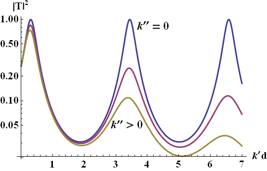
The squared transmission coefficient for a transmission line of length \(d\) and wavenumber \(k_{b}=k^{\prime}+\mathrm{i}k^{\prime\prime}\). If the medium is lossless (blue line), the transmission coefficient reaches maxima at unity. The maxima are equispaced every \(k^{\prime}\Delta d=\pi\), so every half wavelength since \(k=2\pi / \lambda\). With losses the situation changes (magenta and yellow lines). Here, \(k^{\prime\prime}/k^{\prime}=5\%\text{ and }10\%\) have been chosen, respectively. We can see that the maxima get not only lower but also slightly shifted. Note that because of a nonvanishing phase on reflection chosen here as \(\phi_{r}=-0.3\neq0\), the first resonances occur already after a very short distance.

Background: Fabry-Perot Resonances in Nanoantennas

Recent advances in fabrication techniques make it possible to fabricate antennas that can work in the near-infrared and optical frequency bands.

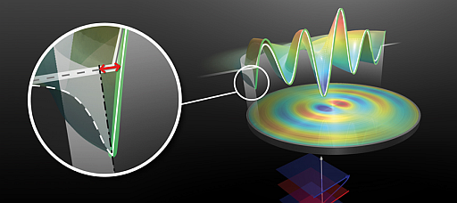
Such antennas can be made of noble metals and are in the order of just a few hundred nanometers. The description of such nanoantennas, however, cannot be made as in the radio frequency domain - metals are not perfect conductors at such short wavelengths and nanoantennas have to be understood in terms of surface plasmon polaritons, collective electron oscillations coupled to light.

Then, the scaling of such antennas can be calculated using the same Fabry-Perot resonance condition that we have just derived! Only the wavenumber is that of a plasmonic mode. \(\phi_{r}\) is the phase accumulated at its reflection at the termination of the antenna.

This approach was used in “Circular Optical Nanoantennas - An Analytical Theory” to understand the characteristics of a kind of antennas that might play an important role in the taylored interaction of light with quantum systems as molecules or quantum dots.

You can see that Fabry-Perot resonances are still very much at the core of scientific activities!

Journal Page | arXiv | PDF

</div>