Tags: Near Field / Far Field / Green's Function
![]() One of the fundamental charge distributions for which an analytical expression of the electric field can be found is that of a line charge of finite length. Nevertheless, the result we will encounter is hard to follow. Two limiting cases will help us understand the basic features of the result.
One of the fundamental charge distributions for which an analytical expression of the electric field can be found is that of a line charge of finite length. Nevertheless, the result we will encounter is hard to follow. Two limiting cases will help us understand the basic features of the result.
Problem Statement
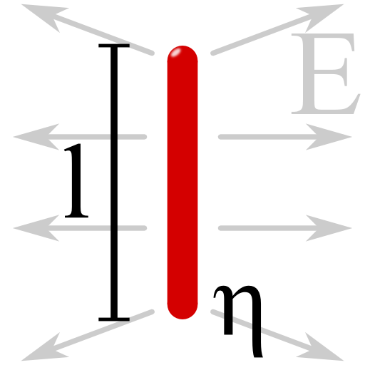
Calculate the electrostatic potential Φ(r) and the electric field E(r) of a line charge with length l. Formally, the charge distribution is given by:

Discuss your result in the limits of infinite line charge, l → ∞ and for large distances |r| ≫ l. For simplicity, restrict yourself in both limiting cases to the x-y-plane.
Hints
Remember that the Dirac delta-distribution δ(r) is defined only in the integral sense,
\[f\left(x_{0}\right)=\int f\left(x\right)\delta\left(x-x_{0}\right)dx\]
Furthermore, the Heaviside step-function might be defined as
\[\Theta\left(x\right) = \begin{cases}1 & x\geq0\\0 & x<0\end{cases}\ .\]
And the Green's function for the Laplace operator Δ is defined by:
\[\Delta_{\mathbf{r}}G\left(\mathbf{r},\mathbf{r}^{\prime}\right)=\delta\left(\mathbf{r}-\mathbf{r}^{\prime}\right)\ .\]
Using the latter definition, can you show that
\[\phi\left(\mathbf{r}\right)=-\frac{1}{\epsilon_{0}}\int G\left(\mathbf{r},\mathbf{r}^{\prime}\right)\rho\left(\mathbf{r}^{\prime}\right)dV^{\prime}\]
is the (formal) solution to the Poisson equation? Specifically, the Greens function for \(\Delta\) can be calculated as
\[\begin{eqnarray*} G\left(\mathbf{r}, \mathbf{r}^{\prime}\right) & = & -\frac{1}{4\pi}\frac{1}{ \left|\mathbf{r}- \mathbf{r}^{\prime}\right|}\ .\end{eqnarray*}\]
The General Solution
First of all, we shall obtain the general potential of a finite line charge. After that we will apply standard techniques to find expressions for the limiting cases we are interested in. In the end we will compare our findings to the general solution graphically.
Using the solution of the Poisson equation in terms of the Green function, we find
\[\begin{eqnarray*}\phi\left(\mathbf{r}\right) & = & \frac{1}{4\pi\epsilon_{0}}\int\frac{\rho\left(\mathbf{r}^{\prime}\right)}{\left|\mathbf{r}-\mathbf{r}^{\prime}\right|}dV^{\prime}\\ & = & \frac{1}{4\pi\epsilon_{0}}\int\int\int\frac{\eta\delta\left(x\right)\delta\left(y\right)\Theta\left(\left|z\right|-l/2\right)}{\left|\mathbf{r}- \mathbf{r}^{\prime}\right|}dx^{\prime}dy^{\prime}dz^{\prime}\\ & = & \frac{\eta}{4\pi\epsilon_{0}}\int_{-l/2}^{l/2}\frac{1}{\sqrt{x^{2}+y^{2}+\left(z-z^{\prime}\right)^{2}}}dz^{\prime} \end{eqnarray*}\]
The last term is a standard integral which we can evaluate as
\[\begin{eqnarray*}\phi\left(\mathbf{r}\right) & = & \frac{\eta}{4\pi \epsilon_{0}} \log \left[\frac{z+ \frac{l}{2}+\sqrt{ \left(z+\frac{l}{2}\right)^{2}+\rho^{2}}}{z-\frac{l}{2}+ \sqrt{\left(z -\frac{l}{2} \right)^{2}+ \rho^{2}}}\right]\ \text{with}\\ \rho & = & \sqrt{x^{2}+y^{2}}\ .\end{eqnarray*}\]
Now this result does not look very intuitive. Let us try to understand it in two limits. First we can consider the limit of an infinitely long line charge, \(l\rightarrow\infty\).
Infinitely Long Line Charge
Of course we cannot simply neglect any term somewhere - we have to thinka little. In the given limit the field cannot depend on the \(z\) axis, an infinitely long charge implies a translation symmetry in this direction. So, without loss of generality we can restrict ourselves to z = 0. Then,
\[\begin{eqnarray*} \phi\left(\rho,z=0,\varphi\right) & = & \frac{\eta}{4\pi\epsilon_{0}} \log\left[\frac{+\frac{l} {2}+ \sqrt{\left(\frac{l}{2}\right)^{2}+\rho^{2}}}{-\frac{l}{2}+\sqrt{\left(\frac{l}{2}\right)^{2}+\rho^{2}}}\right]\\ & = & \frac{\eta}{4\pi\epsilon_{0}}\log\left[\frac{\sqrt{1+\left(2\rho/l\right)^{2}}+1}{\sqrt{1+\left(2\rho/l\right)^{2}}-1}\right]\ . \end{eqnarray*}\]
The latter term in the logarithmic has the form
\[\begin{eqnarray*}\frac{x+1}{x-1} & = & \frac{x^{2}-1}{\left(x-1\right)^{2}}\ ,\ \text{so}\\\phi\left(\rho,z=0,\varphi\right) & = & \frac{\eta}{4\pi\epsilon_{0}}\log\left[\frac{1+\left(2\rho/l\right)^{2}-1}{\left(\sqrt{1+\left(2\rho/l\right)^{2}}-1\right)^{2}}\right]\ .\end{eqnarray*}\]
Now we can see that the term inside the root is very close to unity since \(\rho/l\ll1\). Then, we can try to use the Taylor expansion \(\sqrt{1+x}=1+x/2+\mathcal{O}\left(x^{2}\right)\) and find
\[\begin{eqnarray*}\phi\left(\rho,z=0,\varphi\right) & \approx & \frac{\eta}{4\pi\epsilon_{0}}\log\left[\frac{\left(2\rho/l\right)^{2}}{\left(1+\left(2\rho/l\right)^{2}/2-1\right)^{2}}\right]\\& = & \frac{\eta}{4\pi\epsilon_{0}}\log\left[\frac{4}{\left(2\rho/l\right)^{2}}\right]=\frac{\eta}{2\pi\epsilon_{0}}\log\left[l/\rho\right]\ . \end{eqnarray*}\]
Note that the latter result could have been obtained using a series expansion of the nominator and denominator in the first place. From a general point of view of applicability it is convenient (at least for me) to check if the result can be calculated from as little approximations as possible.
Ok, we have still a little problem to overcome. The argument of the logarithmic is now \(l/\rho\) which is in the studied limit simply zero. However, the potential can be defined up to an arbitrary constant. In our case, it would be \(\propto\log\left(l\right)\) since \(\log\left(l/\rho\right)=\log\left(l\right)-\log\left(\rho\right)\).
Hence we find
\[\begin{eqnarray*} \lim_{l\rightarrow\infty}\phi\left(\mathbf{r}\right) & = & -\frac{\eta}{2\pi\epsilon_{0}}\log\left[\rho\right]\ . \end{eqnarray*}\]
From this result we can see that the electric field has only a ρ component,
\[\begin{eqnarray*}\lim_{l\rightarrow\infty}\mathbf{E}\left(\mathbf{r}\right) & = & -\nabla\left\{ \lim_{l\rightarrow\infty}\phi\left(\mathbf{r}\right)\right\} \\ & = & \frac{\eta}{2\pi\epsilon_{0}}\frac{1}{\rho}\mathbf{e}_{\rho}\ .\end{eqnarray*}\]
The Farfield Limit
Naturally we would like to expand the found potential in some \(l\rightarrow 0\) limit since this equivalent here to \(\left|\mathbf{r} \right|\gg l\). It is useful to look at the behavior again at z = 0 since we have already derived a valuable expression in this case:
\[\begin{eqnarray*} \phi\left(\rho,z=0,\varphi\right) & = & \frac{\eta}{2\pi\epsilon_{0}}\log\left[\frac{2\rho/l}{\sqrt{1+\left(2\rho/l\right)^{2}}-1}\right] \end{eqnarray*}\ .\]
Note that we have used \(\log\left(x^{2}\right)=2\log\left(x\right)\) eliminating the squares in the equaiton. We can again use \(\sqrt{1+x}=1+x/2+\mathcal{O}\left(x^{2}\right)\) but now we have to consider the small variable \(x=l/2\rho\):
\[\begin{eqnarray*} \phi\left( \rho,z=0,\varphi\right) & = & \frac{\eta}{2\pi\epsilon_{0}}\log\left[\frac{1}{ \sqrt{1+\left(l/2\rho\right)^{2}}-l/2\rho}\right]\\ & \approx & -\frac{\eta}{2\pi\epsilon_{0}} \log\left[1+\left(l/2\rho\right)^{2}/2-l/2\rho\right]\ . \end{eqnarray*}\]
Now we see that the term in \(\left(l/\rho\right)^{2}\) can be neglected with respect to the linear counterpart. Further using \(\log\left(1-x\right)\approx-x+\mathcal{O}\left(x^{2}\right)\) we find in first order
\[\begin{eqnarray*}\phi\left(\rho,z=0,\varphi\right) & = & \frac{\eta l}{4\pi\epsilon_{0}}\frac{1}{\rho}\ .\end{eqnarray*}\]
Since the total charge of the line is \(q=\eta l\), this is exactly what we would have expected - the potential of a point charge q and likewise its electric field.
Now what about an arbitrary z? We can try to understand this part in terms of multipole moments without having to calculate anything. From the expression in the xy-plane we already know that the lowest-order term, the electric monopole, is given due to the charge \(q=\eta l\). This behavior is course general - there cannot be any other contribution to this component.
The next-order term, the electric dipole \(\mathbf{p}=\int\mathbf{r}^{\prime}\rho\left(\mathbf{r}^{\prime}\right)dV^{\prime}\) vanishes because of symmetry. So, the next higher-order contribution must be of quadrupolar nature. Hence, for small lenghts of the line charge compared to some probing distance, the approximation as pointcharge seems to be reasonable. Below you can see a comparison of the approximative results we just derived with the full solution.
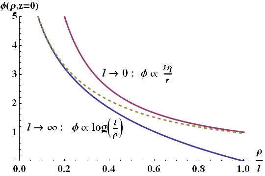
The found electrostatic potential of a line charge. The full solution (yellow dotted line) coincides very nicely with the found approximative solutions for infinite (magenta line) and vanishing length (blue line).
Background: Forces on Molecules by an Everyday Line Charge
If you rub a plastic ruler with one of your shirts, there will be some net charge on both the ruler and your t-shirt. Now you can approach the next tap, make some nice, not too strong, water stream and hold your ruler close to it. You will notice that the water stream changes his way slightly in the direction of the ruler. How can we understand the movement of the water stream?
The reason is that water, \(H_{2}O\), has a permanent dipole moment \(\mathbf{p}\) which is interacting with the local electric field. The interaction potential is given by \(V_{\mathrm{dipole}}\left(\mathbf{r}\right)=-\mathbf{p}\cdot\mathbf{E}\left(\mathbf{r}\right)\) and the force acting on the dipole is the negative gradient of the potential, \(\mathbf{F}\left(\mathbf{r}\right)=-\nabla V\left(\mathbf{r}\right)\). So the force depends on the local derivative of the electric field. Now we can see why the water stream gets diffracted. Furthermore it matters what kind of electric field is present to influence it. We might regard the ruler as a finite line charge. In the solution we will find that the field of a long or short one are in fact different and so is their force on the water stream.
Can you explain what happens to the stream inside a parallel-plate capacitor with assumed constant electric field?